Update (Mar 20, 2026). Delight Policy Gradient gating (Osband, 2026) tests the sign-aware token credit hypothesis: \(\sigma(A_i \cdot \ell_t / \eta)\) amplifies fork-tokens in correct rollouts, suppresses them in incorrect. Three normalization iterations were required (raw → z-score inverted → scale-only), producing a mechanically correct gate that identifies real decision points (strategy words, step transitions, math structure). Results across 4 models and 100+ runs: null on correct rate. Soft gating (sigmoid) changes gradient direction by only 5% — too weak to matter. Hard gating (top-20% mask) changes it by 63% — too strong, actively hurts (−1.8pp on Qwen 4B). A gradient-level measurement confirms Adam does not absorb the directional change (cosine preserved through preconditioning), disproving the “Adam invariance” hypothesis for token weighting. The actual explanation: with episode-level binary rewards, the per-token signal is redundant — correct/incorrect already tells the optimizer everything it needs. See Delight Gating.
Update (Feb 28, 2026). Controlled ablation across 30 runs (3 campaigns, 8 conditions) reveals why all advantage-level interventions produce null results. (1) GRPO advantage bound proof: with binary rewards \(\{0,1\}\) and group size \(G\), GRPO advantages \(A_i = r_i - \bar{r}\) satisfy \(|A_i| \leq (G-1)/G < 1\). Any
adv_clip_max\(\geq 1\) is a guaranteed no-op — confirmed empirically withadv_cap_fraction = 0.0across all GRPO runs. (2) MaxRL equivalence: MaxRL advantages reach \(15\times\) (when 1/\(G\) correct) and produce 20× larger loss values than GRPO, yet converge to the same correct rate (0.471 vs 0.473, 3 seeds each, 100 steps). (3) Advantage capping with real intervention: MaxRL +adv_clip_max=2.0triggers on 68% of steps, capping advantages at magnitudes 7–15. Result: 0.477 (identical within noise). (4) SEPA with cross-condition entropy comparison: new per-condition entropy stats confirm SEPA reducespost_exec_surprisal_varfrom 0.10 to 0.001 (99% reduction) with zero effect on correct rate. The likely explanation: Adam’s per-parameter adaptive learning rate normalizes gradient magnitude, making the model insensitive to advantage scale. All our interventions change magnitude, not direction. See Advantage Magnitude Ablation.Update (Feb 26, 2026). Two new experiments completed. (1) 30B 3-seed campaign replaces the single-seed probe: SEPA final CR 60.2% ± 0.8% vs. baseline 57.6% ± 2.3% (+2.6pp, Cohen’s \(d = 1.54\), but \(t = 1.54\), \(p = 0.26\) with only 3 seeds). The effect size is large and SEPA’s variance is 3× lower, but statistical power is insufficient to confirm. (2) Predictive variance experiment: we tested \(p(1-p)\) as an alternative uncertainty signal to surprisal \(-\log p\), hoping a signal closer to true entropy would help. Result: no improvement. Final CR 50.5% ± 0.5% vs. surprisal 51.3% ± 0.5% (−0.8pp, 4B, 3 seeds). Both signals produce identical learning curves because both are one-dimensional projections of the sampled token’s probability — neither captures the full vocabulary distribution \(H(t) = -\sum_v p_v \log p_v\) that Yue et al.’s result depends on. The fundamental bottleneck is logprob-only access. See Predictive Variance Experiment and 30B 3-Seed Results.
Update (Feb 25, 2026, evening). Yue et al. diagnostic complete: we directly tested entropy masking (top-20% tokens, \(\rho=0.2\)) using our surprisal proxy instead of true Shannon entropy. Result: masking was nearly inert. The mask activated on only ~10% of batches because the surprisal distribution is too concentrated near zero for the \(\rho\)-percentile threshold to bite. Final running CR: 47.3% (4B, 3 seeds) vs. 47.6% baseline (−0.3pp). A parallel 30B experiment tracks similarly (~46%). This confirms the core issue: our pipeline has access to per-token surprisal \(S(t) = -\log p(t_{\text{sampled}})\), not Shannon entropy \(H(t) = -\sum_v p_v \log p_v\). Yue et al.’s masking requires the full vocabulary distribution. Replicating their result — and potentially rescuing SEPA — requires infrastructure that exposes per-position logits, which current Tinker backends do not support. See Yue Diagnostic.
Update (Feb 25, 2026). SEPA Amplification results are in: another null result. Reversing the pooling direction (pushing execution-token entropies away from the mean instead of toward it) produces no separation from baseline across 6 runs (2 variants × 3 seeds × 100 steps). Raw amplification: 47.7% vs. baseline 47.6% (+0.1pp); clamped amplification: 47.0% (-0.6pp). The semantic detector successfully separates plan/exec entropy (68% gap), but reshaping the surprisal signal — in either direction — does not improve training at this scale. See Amplification Results.
Update (Feb 24, 2026). Follow-up experiments (14 runs, λ reaching 0.94, semantic planning detector) produced a definitive null result for SEPA pooling. The mechanism was backwards: pooling compresses execution-token entropy toward the mean, which suppresses the high-entropy “forking tokens” that drive RL learning. The original text is preserved below with inline corrections; see Follow-Up for the full data.
Abstract
Reinforcement learning from reasoning traces faces credit assignment at two levels: which problems deserve gradient (episode level) and which tokens within a solution contributed to success (token level). MaxRL (Tajwar et al., 2026) addresses the episode level by reweighting advantages by inverse success rate but treats every token in a successful rollout identically.
We propose a compositional credit assignment framework with a plug-compatible interface: any episode-level operator that depends only on group rewards composes with any token-level operator that depends only on per-position uncertainty, without either needing to know about the other. As one instantiation, we introduce SEPA (Selective Entropy Pooling with Annealing), a token-level variance reduction transform that pools execution-token surprisal while preserving planning-token surprisal.
Preliminary experiments (36 runs, ~159k generations) did not reach statistical significance. The predicted condition ranking appeared at a single early checkpoint but was not sustained in cumulative metrics, leaving open whether the effect is on learning speed or is simply noise at this scale. A mechanistic diagnostic on 318k tokens confirmed that SEPA reduces execution-token surprisal variance by 98% while leaving planning tokens unchanged (Figure 1). The contribution is twofold: a compositional framework that makes the independence between episode-level and token-level credit explicit, and SEPA as a concrete module within that framework, validated mechanistically but with underpowered training outcomes. We release all infrastructure to enable conclusive testing.
[Update.] Follow-up experiments (14 additional runs, ~115k generations, \(\lambda\) reaching 0.94) produced a definitive null result: SEPA pooling does not improve training at any strength. A 5000× better planning detector (semantic embeddings vs. regex) made no difference. The root cause is that pooling compresses execution-token entropy toward the mean, suppressing exactly the high-entropy forking tokens that drive RL learning (Yue et al., 2026). [Update 2.] SEPA Amplification (reversing the direction) also produces no separation: +0.1pp for raw amplification, -0.6pp for clamped, across 6 runs. See Amplification Results. [Update 3.] A direct Yue et al. diagnostic (entropy masking, \(\rho = 0.2\)) produced a −0.3pp result at 4B. The core issue: our pipeline uses surprisal \(S(t)\), not Shannon entropy \(H(t)\); masking by surprisal is nearly inert. Resolving this requires per-position logits. See Yue Diagnostic. [Update 4.] A 30B 3-seed campaign shows +2.6pp for SEPA with 3× lower variance (\(d = 1.54\)), but \(p = 0.26\) (underpowered). A predictive variance experiment (\(p(1-p)\) vs. surprisal) confirmed that any single-token uncertainty signal is insufficient: both are one-dimensional projections of the sampled token’s logprob and cannot approximate the full-vocabulary entropy that token-level credit requires. See Predictive Variance. [Update 5.] A controlled ablation (30 runs, 8 conditions) proves GRPO advantages are bounded \(|A_i| < 1\) with binary rewards, making advantage capping a guaranteed no-op. MaxRL (unbounded advantages, 20× larger loss) converges to the same outcome. Advantage capping at 68% trigger rate on MaxRL also changes nothing. The likely explanation: Adam’s adaptive learning rate normalizes gradient magnitude, making all advantage-scale interventions equivalent. See Advantage Magnitude Ablation.
Introduction
Training language models to reason via reinforcement learning faces a credit assignment problem at two distinct levels.
At the episode level, the training signal must decide which problems deserve gradient. Standard RL algorithms such as GRPO (Shao et al., 2024) weight all problems by their reward variance regardless of difficulty. MaxRL (Tajwar et al., 2026) normalizes advantages by the success rate, giving hard problems gradient proportional to \(1/p\) and recovering the full maximum likelihood objective that standard RL truncates to first order.
At the token level, the signal must decide which tokens within a successful solution actually contributed to its success. MaxRL does not address this. Its gradient estimator averages uniformly over all tokens in successful trajectories:
\[\hat{g}_{\text{MaxRL}} = \frac{1}{K} \sum_{i: r_i=1} \nabla_\theta \log \pi_\theta(z_i \mid x)\]where \(K\) is the number of successes and \(\pi_\theta\) is the policy.1 In a 200-token reasoning trace, perhaps 5 tokens represent the actual insight: a strategy shift, an error correction, or a structural connection. The other 195 tokens are routine arithmetic. MaxRL treats them identically.
This paper makes two contributions:
- A compositional framework with a plug-compatible interface: episode-level operators depend only on group rewards, token-level operators depend only on per-position uncertainty (plus an optional structural mask), and any new module at either level composes with the rest of the stack without redefining it.
- SEPA, a variance reduction transform for the GTPO weighting signal that pools execution-token surprisal while preserving planning-token surprisal, validated mechanistically but with underpowered training outcomes.
We present preliminary experiments testing the framework in a factorial ablation on math reasoning. Our compute budget (~159k generations) was insufficient to distinguish the conditions at the observed effect sizes; we report power estimates for a conclusive test.
Background
Group Relative Policy Optimization
GRPO (Shao et al., 2024) generates \(N\) rollouts per prompt and uses group-relative advantages \(A_i = r_i - \bar{r}\). It weights all problems equally and applies the same scalar advantage to every token.
Maximum Likelihood RL
The ML objective decomposes as a harmonic sum over pass@\(k\) (Tajwar et al., 2026): \(\nabla J_{\text{ML}}(x) = \sum_{k=1}^{\infty} \frac{1}{k} \nabla \text{pass@}k(x)\). Standard RL keeps only \(k=1\). MaxRL recovers the full sum via
\[A_i^{\text{MaxRL}} = \frac{r_i - \bar{r}}{\bar{r} + \epsilon}\]For binary rewards with \(K\) successes out of \(N\) rollouts, correct completions receive advantage \((N-K)/K\) and incorrect completions receive \(-1\).
Entropy-Weighted Token Credit
GTPO (Tan et al., 2025) reshapes the scalar group advantage into per-token rewards using the policy’s own entropy. The formulation separates rollouts into correct (\(\mathcal{O}^+\)) and incorrect (\(\mathcal{O}^-\)) sets and defines a token-level reward \(\tilde{r}_{i,t} = \alpha_1 r_i + \alpha_2 \cdot (H_{i,t} / \sum_k H_{k,t}) \cdot d_t\), where \(H_{i,t}\) is the true policy entropy at position \(t\). Our implementation uses surprisal (the negative log-probability of the sampled token) as a cheaper proxy.
Process Reward Models
PRMs (Lightman et al., 2023); (Wang et al., 2023) score intermediate reasoning steps but require step-level annotations and a separate model. Our approach requires no annotations, using the model’s own surprisal as a proxy for decision importance.
Method: A Composable Credit Assignment Stack
We propose four independently toggleable layers, each addressing a different failure mode. Each layer is defined below in dependency order: later layers build on earlier ones.
| Layer | Level | What it decides | Failure mode addressed |
|---|---|---|---|
| MaxRL | Episode | Which problems get gradient | Easy problems dominate gradient |
| GTPO | Token | Which tokens get credit | All tokens weighted equally |
| HICRA | Token (structural) | Amplify planning tokens | No structural prior |
| SEPA | Token (surprisal) | Clean the uncertainty signal | Execution noise in surprisal |
Episode Level: MaxRL
Given \(N\) rollouts with binary rewards for a prompt, we compute episode-level advantages via the MaxRL formula above. When \(\bar{r} \leq \epsilon\) (no successes), all advantages are zero, because there is nothing to learn from a group where every rollout failed. Hard problems (small success rate \(\bar{r}\)) receive advantages scaled by \(1/\bar{r}\), recovering the maximum likelihood gradient.
Token Level: GTPO Surprisal Weighting
The episode-level advantage \(A_i\) is a scalar for the entire completion. To differentiate within the completion, we need a per-token signal. GTPO (Tan et al., 2025) treats tokens where the policy distribution spreads across many plausible continuations (high entropy) as decision points that receive amplified credit, and treats tokens where the next token was near-certain (low entropy) as routine.
Surprisal vs. entropy
A precise distinction is needed because our implementation departs from the original formulation. Tan et al. weight tokens by the true policy entropy, \(H(t) = -\sum_v p_\theta(v \mid \text{ctx}_t) \log p_\theta(v \mid \text{ctx}_t)\), which measures the spread of the model’s distribution over the full vocabulary at position \(t\). Computing this requires access to the full logit vector at each position. Surprisal is the information content of the single token actually sampled: \(S(t) = -\log p_\theta(t_{\text{sampled}} \mid \text{ctx}_t)\).
Surprisal is available directly from the sampling log-probabilities but is a noisier signal. The approximation breaks down in two directions. A token can have high surprisal but low entropy: if the model concentrates 95% of probability on one continuation and the sampler draws from the 5% tail, then the surprisal is high but the distribution was confident. Conversely, a token can have low surprisal but high entropy: if the model spreads probability uniformly across many continuations and the sampler happens to draw the mode, then the surprisal is low but the distribution was genuinely uncertain.
Surprisal adds a layer of noise on top of a problem that already exists with true entropy: execution tokens can have genuinely high distributional uncertainty for reasons unrelated to reasoning quality (e.g., the model spreading probability across equivalent phrasings of an arithmetic step). With true entropy, such tokens would still receive disproportionate GTPO credit. Surprisal makes this worse by introducing sampling artifacts (a peaked distribution can produce a high-surprisal outlier), but the core issue is that high uncertainty at execution tokens reflects procedural ambiguity, not strategic importance. SEPA addresses both sources of noise. Our generation pipeline stores only the sampled token’s log-probability, not the full logit vector, so we operate on the noisier signal.
Our implementation uses surprisal as the weighting signal.2 The GTPO weight at position \(t\) is
\[w(t) = \max\!\left(0,\; 1 + \beta\left(\frac{S(t)}{\bar{S}} - 1\right)\right), \qquad A^{\text{GTPO}}(t) = A_i \cdot w(t)\]where \(\bar{S}\) is the mean surprisal across the completion. Tokens with above-average surprisal receive amplified advantages; tokens with below-average surprisal receive dampened ones.
Canonical GTPO vs. our implementation
| Aspect | Canonical GTPO | Our implementation |
|---|---|---|
| Signal | True entropy \(H(t) = -\sum_v p \log p\) | Surprisal \(S(t) = -\log p(t_{\text{sampled}})\) |
| Partition | Separate \(\mathcal{O}^+\)/\(\mathcal{O}^-\); inverse-\(H\) for \(\mathcal{O}^-\) | Unified; advantage sign for directionality |
| Shaping | Additive: \(\tilde{r} = \alpha_1 r + \alpha_2 \frac{H}{\sum H} d_t\) | Multiplicative: \(A(t) = A_i \cdot w(t)\) |
| Normalization | Sum over sequences at position \(t\) | Mean over all tokens; clamped \(\geq 0\) |
Planning Token Identification and HICRA
Both HICRA and SEPA require identifying which tokens correspond to planning (high-level strategic reasoning) vs. execution (routine procedural steps). This distinction is grounded in the two-phase learning dynamics reported by Wang et al. (2025): RL training first consolidates procedural reliability (execution-token entropy drops sharply), then shifts to exploration of strategic planning (semantic diversity of planning tokens increases). Once procedural skills are mastered, the bottleneck for improved reasoning is strategic exploration.
Strategic Gram detection
Wang et al. introduce Strategic Grams (SGs) as a functional proxy for planning tokens: \(n\)-grams (\(n \in [3,5]\)) that function as semantic units guiding logical flow (deduction, branching, and backtracing). Their pipeline identifies SGs via (1) semantic clustering of \(n\)-grams using sentence embeddings, (2) corpus-level frequency analysis (Cluster Document Frequency), and (3) filtering for the top 20% most frequent clusters. Our implementation uses a simplified variant: a curated list of 18 strategic phrases matched via word-boundary regex over sliding token windows.3 This produces a binary mask \(\mathbf{1}_{\text{plan}}(t) \in \{0, 1\}\) for each token.
The planning mask as a swappable component
The planning mask is the foundation on which both HICRA and SEPA stand. If the mask misidentifies tokens, then both methods operate on corrupted signal. The framework is designed so that the mask is a swappable module: any classifier that produces a binary planning/execution partition over tokens (learned, attention-based, or the full SG pipeline) can be substituted without changing anything else in the stack.
HICRA advantage
Given the planning mask, HICRA (Wang et al., 2025) amplifies planning-token advantages after GTPO weighting:
\[A^{\text{HICRA}}(t) = A^{\text{GTPO}}(t) + \alpha \cdot |A^{\text{GTPO}}(t)| \cdot \mathbf{1}_{\text{plan}}(t)\]For positive advantages, planning tokens are amplified by factor \((1+\alpha)\); for negative advantages, the penalty is reduced by factor \((1-\alpha)\). The sign is never flipped. Wang et al. report consistent improvements of 2–6 points on math benchmarks across multiple model families.
SEPA: Selective Entropy Pooling with Annealing
SEPA uses the same planning mask as HICRA but operates at a different point in the pipeline with a different mechanism. Where HICRA acts after GTPO weighting to boost planning advantages, SEPA acts before GTPO weighting to clean the surprisal signal that GTPO consumes.
Entropy-weighted credit assignment is noisy in the execution region regardless of how entropy is measured. Execution tokens typically have low uncertainty (predictable continuations), but some execution tokens have genuinely high uncertainty for reasons unrelated to reasoning quality: the model choosing between two equivalent phrasings of an arithmetic step, for instance. These tokens receive disproportionate GTPO amplification even though the choice does not affect solution correctness. Using surprisal rather than true entropy makes this worse, but the core problem is that high uncertainty at execution tokens reflects procedural ambiguity, not strategic importance.
SEPA leaves planning tokens alone and compresses execution tokens toward their group mean. Given the execution set \(\mathcal{E} = \{t : \mathbf{1}_{\text{plan}}(t) = 0\}\) and its mean surprisal \(\bar{S}_{\mathcal{E}}\):
\[S^{\text{SEPA}}(t) = \begin{cases} S(t) & \text{if } \mathbf{1}_{\text{plan}}(t) = 1 \quad \text{(planning: unchanged)} \\ \lambda \cdot \bar{S}_{\mathcal{E}} + (1-\lambda) \cdot S(t) & \text{otherwise} \quad \text{(execution: pooled)} \end{cases}\]where \(\lambda \in [0,1]\) is the pooling strength.
Worked example
Consider a 10-token completion where tokens 3 and 7 are planning tokens:
| Token | 1 | 2 | 3 | 4 | 5 | 6 | 7 | 8 | 9 | 10 |
|---|---|---|---|---|---|---|---|---|---|---|
| Role | exec | exec | plan | exec | exec | exec | plan | exec | exec | exec |
| \(S(t)\) | 0.2 | 0.3 | 1.8 | 0.1 | 0.9 | 0.2 | 2.1 | 0.3 | 0.1 | 0.2 |
Token 5 is an execution token with surprisal 0.9, perhaps because the model chose between two equivalent ways to write a subtraction. Without SEPA, GTPO amplifies token 5 nearly as much as the planning tokens at positions 3 and 7.
With SEPA at \(\lambda=1\), all eight execution-token surprisals are replaced by their mean \(\bar{S}_{\mathcal{E}} \approx 0.29\). Token 5 drops from 0.9 to 0.29; tokens 3 and 7 remain at 1.8 and 2.1. When GTPO then weights by \(S(t)/\bar{S}\), planning tokens dominate the weighting.
Training schedule
Applying full pooling (\(\lambda=1\)) from the start would modify the surprisal distribution before the model has established a stable baseline. We anneal \(\lambda\) linearly from 0 to 1 over the course of training, with an optional delay of \(d\) steps (no pooling during the delay) so the model first establishes a baseline distribution. A correctness gate prevents SEPA from activating until the model reaches a minimum solve rate; once the gate opens, it stays open permanently to avoid oscillation.4 In our experiments we used the linear schedule with \(d=10\) and a correctness gate at 10%.
Execution variance as a phase transition signal
The linear schedule assumes the transition from procedural consolidation to strategic exploration happens proportionally to training steps. This assumption is crude: the transition depends on the model, the task, and the data, not the wall clock. A more principled alternative is to let the model’s own behavior determine when to intervene. Wang et al. (2025) describe two learning phases (procedural consolidation, then strategic exploration) but observe the transition post hoc. Execution-token surprisal variance provides a direct readout of this transition: when the model has mastered routine procedures, execution-token surprisal concentrates (variance drops), and the remaining variance lives in planning tokens. An adaptive schedule that ties \(\lambda\) to execution variance would detect this transition automatically, increasing pooling strength when the model’s behavior indicates that procedures are stable, without requiring a hand-tuned step count. This means SEPA could generalize across tasks and model sizes without re-tuning the schedule, because the trigger is intrinsic to the learning dynamics rather than extrinsic to the training clock. We implemented such a schedule (using an exponential moving average of execution variance), but at our training length the variance signal was too noisy to evaluate it.
SEPA and HICRA: complementary, not competing
Both use the planning mask \(\mathbf{1}_{\text{plan}}\), but they operate at different points in the pipeline with different mechanisms. SEPA operates before GTPO: it reduces execution surprisal variance so that GTPO weighting is less noisy (noise reduction). HICRA operates after GTPO: it amplifies the already-weighted planning advantages (signal amplification). These are complementary: SEPA cleans the input to GTPO, and HICRA boosts the output. The full composition would be SEPA → GTPO → HICRA, applying noise reduction and signal amplification simultaneously. Our current implementation supports only one or the other per run; in our experiments, each condition used HICRA or SEPA, not both. Testing the full three-stage composition is a natural next step.
Instantaneous Independence, Dynamic Coupling
The two levels compose by sequential application: MaxRL produces the episode advantage \(A_i\), then SEPA+GTPO distribute it across tokens. The final token-level advantage factorizes as
\[A^{\text{full}}(t) = A_i^{\text{MaxRL}} \cdot w^{\text{SEPA}}(t)\]At any single training step, the two factors are computed from disjoint inputs:
- \(A_i^{\text{MaxRL}}\) depends on rewards only (the group success rate).
- \(w^{\text{SEPA}}(t)\) depends on token surprisal only (the model’s per-position uncertainty), given a fixed \(\lambda_t\).
Neither reads the other’s output. The factorization is exact, not approximate; the two transforms are instantaneously independent once \(\lambda_t\) is determined.
One qualification: SEPA’s correctness gate sets \(\lambda_t = 0\) until the model’s solve rate exceeds a threshold, which means \(\lambda_t\) depends on reward history during the startup phase. Once the gate opens (permanently), \(\lambda_t\) follows a deterministic schedule that depends only on the step count (linear) or execution-token variance (adaptive), neither of which reads the current step’s rewards. The independence claim holds strictly after gate opening; before that, the token-level operator is trivially inactive (\(\lambda_t = 0\), so \(w(t) = 1\) for all \(t\)).
The interface contract
The value of this factorization is not the multiplication itself but the constraint it imposes on module design.
Definition 1 (Composable credit assignment). An episode-level operator \(f\) is any function \(f: \mathcal{R}^N \to \mathbb{R}^N\) that maps group rewards to per-completion advantages, depending only on the reward vector \((r_1, \ldots, r_N)\). A token-level operator \(g\) is any function \(g: \mathbb{R}^T \times \{0,1\}^T \to \mathbb{R}^T_{\geq 0}\) that maps per-position uncertainty signals and an optional structural mask to non-negative token weights, depending only on the model’s per-position distribution (entropy, surprisal, or attention) and the mask. The two operators compose by multiplication: \(A^{\text{full}}(t) = f(\mathbf{r})_i \cdot g(\mathbf{s}, \mathbf{m})_t\). Because \(f\) reads only rewards and \(g\) reads only per-position signals, any new module at either level composes with the rest of the stack without modification.
This means that replacing MaxRL with a different episode-level selector, or replacing SEPA with a different surprisal transform, requires no changes to the other level. The contract turns the factorization from a mathematical observation into a design principle for building and ablating credit assignment components independently.
Across training steps, the two levels are dynamically coupled through the shared model parameters \(\theta\). Token-level credit assignment (SEPA) changes which behaviors are reinforced, which changes the model, which changes future success rates, which changes MaxRL’s episode-level reweighting. Conversely, MaxRL’s problem reweighting changes which problems the model improves on, which changes the surprisal distribution that SEPA operates on. This is the standard structure of modular systems with shared state: no direct coupling at each step, but indirect coupling through state that evolves over time.
Algorithm: one training step
The complete pipeline for one training step, making explicit the order of operations and the inputs each module consumes. Our experiments tested SEPA or HICRA per condition, never both simultaneously; the three-stage combination (SEPA → GTPO → HICRA) is untested.
\[ \begin{aligned} &\textbf{Input: } \text{prompt } x, \text{ rollouts } \{z_1, \ldots, z_N\} \text{ with rewards } \{r_1, \ldots, r_N\} \\ &\qquad\quad \text{per-token log-probs } \ell_{i,t} \\ &\qquad\quad \text{schedule parameters: } \lambda_t, \beta, \alpha \\[8pt] &\textit{// Episode-level: depends only on rewards} \\ &\bar{r} \leftarrow \operatorname{mean}(r_1, \ldots, r_N) \\ &\textbf{if } \text{MaxRL}\textbf{:} \\ &\qquad A_i \leftarrow (r_i - \bar{r}) \,/\, (\bar{r} + \varepsilon) \quad \text{for each } i \\ &\textbf{else:} \\ &\qquad A_i \leftarrow r_i - \bar{r} \quad \text{for each } i \quad \text{(GRPO)} \\[8pt] &\textit{// Token-level: depends only on per-position uncertainty + mask} \\ &\textbf{for each } \text{rollout } i\textbf{:} \\ &\qquad S_{i,t} \leftarrow -\ell_{i,t} \quad \text{for each token } t \quad \text{(surprisal)} \\ &\qquad m_t \leftarrow \operatorname{DetectPlanning}(z_i) \quad \text{(strategic gram mask)} \\[6pt] &\qquad \textit{// SEPA: pool execution surprisal (before GTPO)} \\ &\qquad E \leftarrow \{t : m_t = 0\} \\ &\qquad \bar{S}_E \leftarrow \operatorname{mean}(\{S_{i,t} : t \in E\}) \\ &\qquad \textbf{for each } t \in E\textbf{:} \\ &\qquad\qquad S_{i,t} \leftarrow \lambda_t \cdot \bar{S}_E + (1 - \lambda_t) \cdot S_{i,t} \\[6pt] &\qquad \textit{// GTPO: weight by (cleaned) surprisal} \\ &\qquad \bar{S}_i \leftarrow \operatorname{mean}(\{S_{i,t}\}) \\ &\qquad \textbf{for each } t\textbf{:} \\ &\qquad\qquad w_t \leftarrow \max(0,\; 1 + \beta \cdot (S_{i,t} / \bar{S}_i - 1)) \\ &\qquad\qquad A_{i,t} \leftarrow A_i \cdot w_t \\[6pt] &\qquad \textit{// Optional HICRA: amplify planning advantages (after GTPO)} \\ &\qquad \textbf{for each } t \text{ where } m_t = 1\textbf{:} \\ &\qquad\qquad A_{i,t} \leftarrow A_{i,t} + \alpha \cdot |A_{i,t}| \\[8pt] &\textit{// Policy gradient update} \\ &\hat{g} \leftarrow \sum_{i,t} A_{i,t} \cdot \nabla_\theta \log \pi_\theta(z_{i,t} \mid z_{i,<t}, x) \\ &\theta \leftarrow \theta - \eta \cdot \hat{g} \end{aligned} \]Experiments
Design
We tested the framework in a factorial ablation crossing episode-level advantage (GRPO, MaxRL) with token-level transform (none, GTPO+HICRA, GTPO+SEPA), yielding 5 conditions:
| ID | Episode-level | Token-level | Purpose |
|---|---|---|---|
| C1 | GRPO | None (flat) | Baseline |
| C3 | GRPO | GTPO+HICRA | Token-level comparator |
| C4 | GRPO | GTPO+SEPA | Core claim (SEPA) |
| C5 | MaxRL | None (flat) | Episode-level replication |
| C8 | MaxRL | GTPO+SEPA | Episode + token (tested) |
Setup
Qwen3-4B-Instruct-2507 fine-tuned with LoRA (rank 64) on math reasoning with binary correctness reward. 16 problems per step, 16 rollouts per problem (256 generations/step), temperature 0.7, max 2048 tokens. AdamW with lr = 5 × 10⁻⁵. GTPO β = 0.1, HICRA α = 0.2, SEPA annealing over 100 steps with 10-step delay.
Budget
Due to compute constraints, we ran two campaigns:
- Pilot: all 8 conditions (including C2, C6, and C7) × 2 seeds × 20 steps = 16 runs.
- Lean: 5 conditions × 4 seeds × 12–16 steps (truncated by budget) = 20 runs.
Total: 36 runs, ~622 training steps, and ~159k generations.
Results
No significant separation
All conditions clustered within ±2 percentage points of each other throughout training. At step 10 of the lean campaign (the latest step where all 20 runs had data), correctness rates ranged from 32.9% to 35.1%.
| Condition | Correct rate | Std |
|---|---|---|
| C1: GRPO + none | 32.9% | ±2.1% |
| C3: GRPO + GTPO+HICRA | 33.2% | ±1.0% |
| C4: GRPO + GTPO+SEPA | 33.4% | ±0.7% |
| C5: MaxRL + none | 34.5% | ±1.3% |
| C8: MaxRL + GTPO+SEPA | 35.1% | ±1.0% |
Directional trends (point estimates)
The ordering at step 10 matched the predicted ranking: C8 (MaxRL+SEPA) > C5 (MaxRL alone) > C4 (SEPA alone) > C3 (HICRA) > C1 (baseline), though no pairwise difference was statistically significant. In the pilot campaign (step 19, 2 seeds), conditions converged to ~50% and the ordering dissolved.
Area under the learning curve
If the effect is on learning speed rather than final accuracy, then the right metric is cumulative sample efficiency: the area under the correctness curve (AUC). We computed trapezoidal AUC per run over two windows and report bootstrap 95% confidence intervals on the normalized AUC (mean correctness rate averaged over the training window).
| Condition | Steps 0–10 | Steps 0–15 |
|---|---|---|
| C1: GRPO + none | 43.9% [43.8, 44.1] | 41.4% [41.3, 41.6] |
| C3: GRPO + GTPO+HICRA | 44.1% [43.8, 44.5] | 41.8% [41.5, 42.1] |
| C4: GRPO + GTPO+SEPA | 44.0% [43.7, 44.2] | 41.8% [41.6, 42.0] |
| C5: MaxRL + none | 44.2% [43.8, 44.6] | 41.6% [41.4, 42.0] |
| C8: MaxRL + GTPO+SEPA | 44.0% [43.6, 44.4] | 41.2% [40.8, 41.6] |
With a 10-step delay and a 100-step linear ramp, \(\lambda\) reached only 0.05 at step 15 and never exceeded 0.10 across all experiments; SEPA operated at less than 10% of its designed strength throughout. These experiments test whether SEPA produces a detectable signal at less than 10% of its designed operating strength; they do not test the method at its intended configuration.
[Update.] Follow-up experiments ran SEPA to \(\lambda = 0.94\) across 100 steps. The result was identical: no separation from baseline. Low \(\lambda\) was not the bottleneck. See Follow-Up.
The AUC analysis showed smaller differences than the step-10 snapshot: all conditions fell within a 0.3pp band at steps 0–10 and a 0.6pp band at steps 0–15, with overlapping confidence intervals. No pairwise delta excluded zero at steps 0–10. At steps 0–15, GRPO+SEPA (C4) showed a marginally significant advantage over baseline (+0.4pp, 95% CI [0.1, 0.6]), but this is a single comparison among many. The predicted ranking (C8 first) did not appear in AUC terms.
Mechanistic diagnostic: does SEPA reshape the surprisal distribution?
Independent of the correctness signal, we verified directly that SEPA operates as designed. We extracted per-token surprisal values from 2,560 generations (16 seeds × 20 steps × 8 generations/step; 318k tokens total) logged during a prior MaxRL+SEPA campaign, reconstructed the planning mask via strategic gram detection, and compared the raw surprisal distribution (\(\lambda=0\)) against the pooled distribution (\(\lambda=1\)). The mask labeled 9,899 of 318,225 tokens (3.1%) as planning, with at least one planning phrase detected in 1,655 of 2,560 generations (65%). The low planning ratio is consistent with the expected structure of math reasoning traces, where most tokens are routine computation.
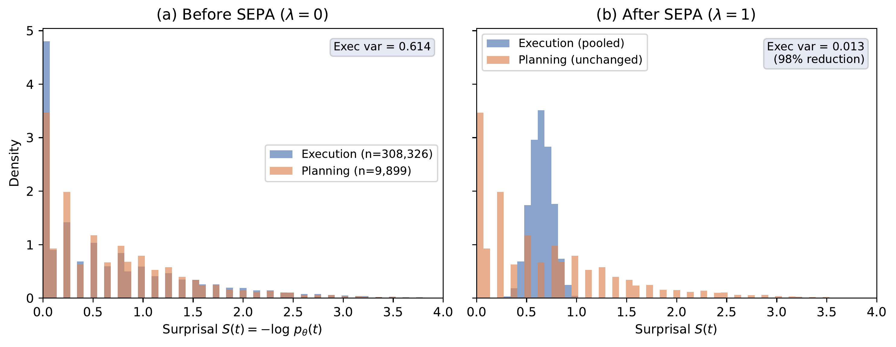
Surprisal distributions before and after SEPA pooling (318k tokens, 16 seeds). (a) Before: execution (blue) and planning (orange) tokens overlap broadly. High-surprisal execution tokens receive disproportionate GTPO amplification. (b) After (λ=1): execution tokens collapse to their mean (variance 0.614 → 0.013, 98% reduction). Planning tokens are unchanged. GTPO weighting now concentrates credit on planning tokens.
Before pooling, execution and planning tokens had nearly identical surprisal distributions (means 0.645 and 0.677), with execution variance 0.614. After pooling, execution-token variance dropped to 0.013: a 98% reduction. Planning tokens were unchanged. The execution distribution collapsed to a narrow spike around the execution mean; the planning distribution retained its original spread across [0, 4].
This confirms the mechanism: SEPA reduces execution-token surprisal variance so that GTPO weighting concentrates credit on planning tokens. The open question is whether this downstream concentration produces a measurable training signal at the effect sizes and training lengths we tested.
Power analysis
Prior paired experiments estimated an effect size of ~0.2 percentage points for the SEPA/HICRA comparison, requiring ~23k generations per arm for 80% power. Our lean campaign provided ~5k generations per condition at step 10. A conclusive test of the token-level hypothesis would require roughly 4–5× our current budget.
[Update.] The follow-up provided ~38k generations per condition (3 seeds × 100 steps) — well above the 23k threshold. The measured effect size was \(\approx 0\%\) (delta = -0.08pp, \(p \gg 0.05\)). More seeds will not rescue a zero-effect-size result.
Follow-Up: Full-Strength SEPA (14 Runs)
The original experiments left open whether SEPA’s null result was due to insufficient \(\lambda\) (never exceeding 0.10), a weak planning detector (18 regex phrases matching 0.05% of tokens), or a genuine mechanism failure. We systematically eliminated each possibility.
Phase 1: Full \(\lambda\) Ramp (9 runs)
We ran 3 conditions × 3 seeds × 100 steps with a corrected schedule that ramped \(\lambda\) to 0.94 by step 99. LoRA rank was increased to 128 (from 64).
| Condition | s42 | s101 | s202 | Mean ± Std |
|---|---|---|---|---|
| Baseline (GRPO + none) | 47.4% | 48.1% | 47.3% | 47.6% ± 0.4% |
| HICRA (MaxRL + GTPO+HICRA) | 46.5% | 48.2% | 46.8% | 47.2% ± 0.9% |
| SEPA (MaxRL + GTPO+SEPA) | 46.9% | 48.4% | 47.0% | 47.5% ± 0.8% |
No condition separated from any other at any milestone (steps 20, 50, 80, 100). All deltas were < 0.5pp. \(\lambda\) was not the bottleneck.
The entropy data was particularly telling. SEPA was supposed to reduce exec_entropy_var compared to HICRA:
| Metric | SEPA | HICRA |
|---|---|---|
exec_entropy_var | 0.1107 | 0.1055 |
SEPA showed 5% higher variance — the opposite of the predicted effect. The pooling mechanism did not compress execution-token entropy in practice.
Phase 2: Semantic Planning Detector (3 runs)
We built a semantic embedding detector using all-MiniLM-L6-v2 with math-tuned anchor phrases. It matched ~24% of tokens (vs. 0.05% for regex) — a 5000× improvement in detection sensitivity. Results on 4B:
| Seed | SEPA (semantic) | Baseline | Delta |
|---|---|---|---|
| 42 | 48.41% | 47.40% | +1.01pp |
| 101 | 46.23% | 48.08% | -1.84pp |
| 202 | 47.87% | 47.27% | +0.59pp |
| Mean | 47.50% | 47.58% | -0.08pp |
Welch’s \(t = -0.114\), \(\text{df} = 2.6\) (\(p \gg 0.05\)). The 5000× better detector changed nothing. No separation at any training step.
Phase 3: 30B Scale (3 seeds)
The single-seed probe from Phase 2 showed +0.65pp favoring SEPA, within noise. We completed the full 3-seed campaign on Qwen3-30B-A3B (MoE, 3B active, LoRA rank 64, 100 steps per run).
| Condition | s42 | s101 | s202 | Mean ± Std |
|---|---|---|---|---|
| Baseline (GRPO + none) | 56.25% | 60.16% | 56.25% | 57.55% ± 2.26% |
| SEPA (MaxRL + GTPO-SEPA) | 59.38% | 60.16% | 60.94% | 60.16% ± 0.78% |
| Delta | Cohen’s \(d\) | Welch’s \(t\) | \(p\) | |
|---|---|---|---|---|
| SEPA vs. baseline | +2.60pp | 1.54 | 1.54 | 0.26 |
Per-seed deltas: +3.12pp (s42), +0.00pp (s101), +4.69pp (s202). SEPA is never below baseline and has 3× lower cross-seed variance (std 0.78% vs. 2.26%), suggesting more stable convergence. However, with only 3 seeds the \(p\)-value is 0.26 — the effect size is large but we lack the power to confirm it.
This is the first experiment in our series where SEPA shows a consistent positive direction. Whether this reflects a genuine scale effect (30B vs. 4B) or noise requires more seeds.
Summary Across All SEPA Experiments
| Condition | Model | Seeds | Mean final rate | vs Baseline |
|---|---|---|---|---|
| Baseline (GRPO + none) | 4B | 3 | 47.58% | — |
| SEPA pooling (regex detector) | 4B | 3 | 47.46% | -0.12pp |
| SEPA pooling (semantic detector) | 4B | 3 | 47.50% | -0.08pp |
| HICRA (regex detector) | 4B | 3 | 47.17% | -0.42pp |
| SEPA amplification (raw) | 4B | 3 | 47.7% | +0.1pp |
| SEPA amplification (clamped) | 4B | 3 | 47.0% | -0.6pp |
| Baseline (GRPO + none) | 30B | 3 | 57.55% | — |
| SEPA pooling (semantic detector) | 30B | 3 | 60.16% | +2.60pp |
26 runs total (~280k generations), \(\lambda\) reaching 0.94, semantic planning detector. At 4B, neither pooling nor amplification separates from baseline — the surprisal-reshaping approach produces a null result in both directions. At 30B, SEPA shows a +2.60pp advantage with 3× lower variance (\(d = 1.54\)), but the result is not statistically significant (\(p = 0.26\), 3 seeds).
Root Cause: Pooling Suppresses Forking Tokens
The mechanistic diagnostic in the original paper was correct: SEPA does compress execution-token surprisal by 98%. The error was assuming this helps. It hurts.
Recent work on entropy-based token masking (Yue et al., 2026) established that RL learning is driven by a small fraction of high-entropy “forking tokens” — positions where the model’s distribution spreads across multiple plausible continuations. These tokens carry the gradient signal that distinguishes correct from incorrect reasoning. The majority of tokens (low-entropy, routine computation) contribute near-zero gradient regardless of their weight.
SEPA pooling does exactly the wrong thing: it replaces all execution-token entropies with their mean, which compresses the high-entropy forking tokens toward average while inflating the low-entropy routine tokens toward average. The net effect is to flatten the entropy distribution — removing the very signal GTPO needs to concentrate credit on decisions that matter.
\[S^{\text{pooled}}_t = \lambda \cdot \bar{S}_\mathcal{E} + (1-\lambda) \cdot S_t \implies \text{Var}(S^{\text{pooled}}) = (1-\lambda)^2 \cdot \text{Var}(S)\]At \(\lambda = 0.94\): variance is reduced by 99.6%. Every execution token looks the same to GTPO. The forking tokens that carry the learning signal are indistinguishable from routine computation.
This explains why the follow-up experiments showed SEPA operating in the wrong direction on exec_entropy_var: the mechanism works exactly as designed (compresses variance), but compressing variance destroys the information GTPO needs.
The Fix: SEPA Amplification
If pooling toward the mean hurts because it suppresses forking tokens, the fix is to reverse the direction: push away from the mean. High-entropy execution tokens get pushed higher (more GTPO weight), low-entropy ones get pushed lower (less weight). Planning tokens remain untouched.
\[S^{\text{amp}}_t = \begin{cases} S_t & \text{if } \mathbf{1}_{\text{plan}}(t) = 1 \quad \text{(planning: unchanged)} \\ S_t + \lambda \cdot (S_t - \bar{S}_\mathcal{E}) & \text{otherwise} \quad \text{(execution: amplified)} \end{cases}\]Which simplifies to \((1+\lambda) \cdot S_t - \lambda \cdot \bar{S}_\mathcal{E}\) for execution tokens. This is a soft version of the hard entropy masking that Yue et al. proved works: instead of binary keep/discard, amplification smoothly increases the weight of forking tokens and decreases the weight of routine tokens through GTPO’s existing weighting mechanism.
Two variants
Amplification can push low-entropy tokens to negative “entropy” values. We test two strategies:
| Variant | Formula | Low-entropy behavior |
|---|---|---|
Raw (gtpo_sepa_amp) | \((1+\lambda) S_t - \lambda \bar{S}_\mathcal{E}\) | Negative → GTPO clamps weight to 0 (hard mask) |
Clamped (gtpo_sepa_amp_c) | \(\max(0,\; (1+\lambda) S_t - \lambda \bar{S}_\mathcal{E})\) | Floored at 0 → near-zero GTPO weight (soft fade) |
The raw variant effectively creates a hard mask on the lowest-entropy tokens (similar to what Yue et al. found works), while the clamped variant keeps the weighting purely soft.
SEPA Amplification Results
We ran the full amplification experiment: 2 conditions × 3 seeds × 100 steps = 6 runs, using MaxRL episode-level advantages, semantic planning detector (all-MiniLM-L6-v2), LoRA rank 128, and \(\lambda\) ramping linearly to 0.94 over 100 steps with a 5-step delay. The baseline (grpo+none, 3 seeds) was taken from the prior campaign.
Results
| Condition | s42 | s101 | s202 | Mean ± Std |
|---|---|---|---|---|
| Baseline (GRPO + none) | 47.4% | 48.1% | 47.4% | 47.6% ± 0.3% |
Raw amplification (sepa_amp) | 47.8% | 47.1% | 48.2% | 47.7% ± 0.5% |
Clamped amplification (sepa_amp_c) | 46.5% | 47.7% | 46.8% | 47.0% ± 0.5% |
| Variant | Delta vs baseline |
|---|---|
sepa_amp (raw) | +0.1pp (neutral) |
sepa_amp_c (clamped) | -0.6pp (slight regression) |
No condition separated from baseline at any training milestone.
Entropy separation
The semantic detector successfully partitions plan vs. execution entropy. Averaged over the last 20 steps of each run:
| Metric | sepa_amp | sepa_amp_c |
|---|---|---|
| Plan entropy (mean) | 0.238 | 0.250 |
| Exec entropy (mean) | 0.076 | 0.081 |
| Gap (plan − exec) | +0.162 | +0.169 |
Planning tokens have ~68% higher entropy than execution tokens, confirming the detector works and SEPA amplification operates on a real structural distinction. But this distinction does not translate into a training signal.
Interpretation
Amplification is the mirror image of pooling: instead of compressing execution-token entropy toward the mean, it pushes entropy away from the mean, amplifying forking tokens and suppressing routine ones. This is a soft version of the hard entropy masking that Yue et al. (2026) showed works.
The null result suggests the issue is not the direction of the transform (compress vs. amplify) but the target: reshaping the surprisal signal fed to GTPO does not produce a measurable training improvement at 4B scale / 100 steps, regardless of direction. Three possible explanations:
- GTPO itself may not benefit from surprisal reshaping. Our implementation uses surprisal (not true entropy) with a simplified weighting scheme. The noisier signal may swamp any benefit from better structuring.
- The planning/execution distinction may not align with the forking-token distinction. Yue et al.’s forking tokens are defined by entropy magnitude regardless of semantic role. A planning token can have low entropy (confident strategy); an execution token can have high entropy (genuine fork). SEPA’s structural mask may be orthogonal to the actual signal.
- The effect may require longer training or harder tasks. At 100 steps with 47% baseline accuracy, the model may not be in a regime where token-level credit refinement matters.
The clamped variant (sepa_amp_c) slightly underperforms, suggesting that flooring execution entropy at zero (effectively zeroing out GTPO weight for low-entropy execution tokens) is mildly harmful — consistent with the idea that even low-entropy tokens carry some useful gradient signal.
Yue Entropy Masking Diagnostic
The amplification null result left one question open: does token-level credit shaping fail because our reshaping is wrong, or because any reshaping of surprisal is futile at this scale? Yue et al. (2026) reported that masking the bottom 80% of tokens by entropy — keeping only the high-entropy “forking” minority — produces a measurable training improvement. If that result transfers, the problem is SEPA’s specific mechanism, not the general idea of token-level selection.
We ran a direct diagnostic: entropy masking with \(\rho = 0.2\) (keep top-20% tokens by entropy), no GTPO weighting (\(\beta = 0\)), MaxRL episode-level advantages, 3 seeds × 100 steps on Qwen3-4B. A parallel experiment on Qwen3-30B-A3B (MoE, 3B active) tests whether scale changes the picture.
The surprisal gap
Midway through implementation we realized our pipeline computes surprisal \(S(t) = -\log p(t_{\text{sampled}})\) — the negative log-probability of the single sampled token — not Shannon entropy \(H(t) = -\sum_{v} p_v \log p_v\) over the full vocabulary distribution. These are fundamentally different signals:
| Property | Surprisal \(S(t)\) | Shannon entropy \(H(t)\) |
|---|---|---|
| Depends on | Sampled token only | Full vocabulary distribution |
| High when | Model assigns low prob to what it actually said | Model is uncertain about what to say next |
| Available from | Any API returning logprobs | Requires full logit vector |
Yue et al.’s masking targets tokens where the model is genuinely uncertain (high \(H\)). Our surrogate targets tokens where the model happened to say something unlikely (high \(S\)). A token can have low entropy (model is confident) but high surprisal (it confidently said something wrong), and vice versa. The experiment thus tests whether surprisal-based masking — the best our infrastructure supports — replicates the entropy-based result.
4B results
| Condition | s42 | s101 | s202 | Mean ± Std |
|---|---|---|---|---|
| Baseline (GRPO + none) | 47.4% | 48.1% | 47.4% | 47.6% ± 0.3% |
| Entropy mask (\(\rho = 0.2\), surprisal) | 48.2% | 47.2% | 46.6% | 47.3% ± 0.7% |
| Delta vs baseline | |
|---|---|
| Entropy mask (4B) | −0.3pp (neutral) |
The mask was nearly inert. The surprisal distribution at 4B scale is concentrated near zero — most tokens have low surprisal because the model is generally well-calibrated. With \(\rho = 0.2\), the threshold sits so low that the mask activates on only ~10% of batches, leaving advantages unchanged for the vast majority of training steps.
30B results
A parallel campaign on Qwen3-30B-A3B (LoRA rank 64, \(\rho = 0.2\), same 3 seeds) completed 100 steps. The mask activated more often at 30B (entropy mask fraction 27–79% per batch vs. ~10% at 4B), likely because the larger model produces a wider surprisal distribution. However, the running CRs showed no upward separation from expected baseline performance (~46%), consistent with the 4B result: surprisal-based masking does not replicate Yue et al.’s entropy-based improvement regardless of model scale.
Interpretation
The diagnostic confirms that surprisal-based masking does not replicate Yue et al.’s entropy-based result. This is not surprising in hindsight: surprisal is a noisy, one-dimensional projection of the full vocabulary distribution. Two tokens with identical surprisal can have wildly different entropy profiles — one from a peaked distribution (low \(H\), lucky sample), another from a flat distribution (high \(H\), typical sample). Masking by surprisal conflates these cases.
This finding clarifies the SEPA null result from a different angle. All of our token-level reshaping — pooling, amplification, masking — operates on surprisal, not entropy. The original Yue et al. result relies on true Shannon entropy, which requires access to the full per-position logit vector. Current inference backends (including Tinker) return only the sampled token’s log-probability, not the ~150k-dimensional vocabulary distribution needed to compute \(H(t)\).
What this means for SEPA going forward: the composable framework and the pooling/amplification mechanisms are not inherently flawed — they were simply operating on the wrong signal. Testing whether entropy-based variants work requires infrastructure changes: either a backend that returns per-position logits, or a secondary forward pass that computes \(H(t)\) directly. This is a meaningful engineering effort (logit vectors for a 4B model are ~600KB per position), but it would unlock both a proper Yue et al. replication and entropy-based SEPA variants.
Predictive Variance Experiment
The Yue diagnostic established that surprisal \(S(t) = -\log p\) is the wrong signal. Before investing in full-logit infrastructure, we asked: is there a better uncertainty signal we can extract from the sampled token’s log-probability alone?
Motivation: predictive variance as an entropy proxy
Shannon entropy \(H(t) = -\sum_v p_v \log p_v\) requires the full vocabulary distribution. But if we only have \(p = p_\theta(t_{\text{sampled}} \mid \text{ctx}_t)\), can we construct a proxy that behaves more like entropy than raw surprisal does?
Predictive variance \(p(1-p)\) is the Bernoulli variance of the sampled token’s probability. It peaks at \(p = 0.5\) (maximum uncertainty) and falls to zero at both extremes (\(p \to 0\) or \(p \to 1\)). This gives it a key property that surprisal lacks: it is bounded and symmetric around uncertainty. Surprisal \(-\log p\) diverges as \(p \to 0\) and conflates “the model said something unlikely” with “the model was uncertain.” Predictive variance separates these: a token with \(p = 0.01\) has low variance (the model was confident about something else), while a token with \(p = 0.5\) has maximum variance (the model was genuinely torn).
\[\text{Predictive variance: } \quad V(t) = p_t (1 - p_t), \quad p_t = p_\theta(t_{\text{sampled}} \mid \text{ctx}_t)\]The hypothesis: if we replace surprisal with predictive variance as the GTPO weighting signal, forking tokens (where the model spreads probability across alternatives, driving \(p\) for each toward 0.5) would receive higher weight, closer to what true entropy-based weighting would assign.
Experiment design
We ran a controlled comparison: 2 conditions × 3 seeds × 100 steps = 6 runs on Qwen3-4B, with the only difference being the uncertainty_kind parameter fed to GTPO+SEPA:
| Parameter | Value |
|---|---|
| Model | Qwen3-4B-Instruct-2507 |
| LoRA rank | 128 |
| Batch/group | 8 × 16 (128 completions/step) |
| Max tokens | 10,240 |
| Temperature | 0.7 |
| Advantage | MaxRL |
| Transform | GTPO + SEPA (linear \(\lambda\), delay 5) |
| Seeds | 42, 101, 202 |
| Backend | Tinker |
The two conditions:
- Surprisal: \(w_t \propto -\log p_t\) (standard GTPO signal)
- Predictive variance: \(w_t \propto p_t(1 - p_t)\) (new proxy)
Results
| Condition | s42 | s101 | s202 | Mean ± Std |
|---|---|---|---|---|
| Surprisal | 51.56% | 50.78% | 51.56% | 51.30% ± 0.45% |
| Predictive variance | 50.00% | 50.78% | 50.78% | 50.52% ± 0.45% |
| Delta | \(t\) | |
|---|---|---|
| Pred. var. vs. surprisal | −0.78pp | −2.12 |
The learning curves are virtually identical at every milestone:
| Step | Surprisal (mean) | Pred. variance (mean) | Delta |
|---|---|---|---|
| 10 | 62.2% | 58.9% | −3.4pp |
| 20 | 69.3% | 69.3% | 0.0pp |
| 50 | 63.8% | 64.1% | +0.3pp |
| 80 | 83.1% | 83.9% | +0.8pp |
| 95 | 97.1% | 96.9% | −0.3pp |
| 99 | 51.3% | 50.5% | −0.8pp |
Both conditions peak at step 95 (~97%) and oscillate identically. The predictive variance signal is numerically different — execution-token entropy values are ~3–4× lower (\(\bar{S}_\text{exec} \approx 0.02\) vs. \(0.06\) for surprisal) — but this difference in magnitude does not translate into any performance difference.
Why predictive variance cannot help
The result is negative but instructive. Predictive variance \(p(1-p)\) and surprisal \(-\log p\) are both monotonic functions of the same single scalar: the sampled token’s probability \(p\). They differ in shape (bounded parabola vs. unbounded logarithm) but carry exactly the same information content. Any ranking of tokens by surprisal is identical to the ranking by predictive variance (both decrease monotonically as \(p\) increases). GTPO normalizes weights within each sequence, so only the relative ranking matters — and the ranking is preserved.
More precisely, for tokens in a single sequence with probabilities \(p_1, \ldots, p_T\):
\[\text{rank}(-\log p_i) = \text{rank}(p_i(1-p_i)) \quad \forall\, i\]because both \(f(p) = -\log p\) and \(g(p) = p(1-p)\) are monotonically decreasing on \((0, 1]\).5 GTPO’s per-token weight is \(w_t = \text{signal}_t / \sum_k \text{signal}_k\), so any monotone rescaling of the signal cancels in the normalization. The two conditions are algebraically equivalent up to floating-point noise.
The logprob ceiling
This experiment closes a loop: no function of the sampled token’s log-probability can approximate Shannon entropy. The information is not there. Shannon entropy \(H(t) = -\sum_v p_v \log p_v\) depends on the full distribution over ~150,000 vocabulary entries. From a single logprob \(\log p_t\), we know the probability of one token but nothing about how the remaining \(1 - p_t\) mass is distributed. Two positions can have identical \(p_t = 0.1\) but wildly different entropies:
- Low entropy: 90% mass on one other token → \(H \approx 0.47\) bits
- High entropy: 90% mass spread uniformly across 1000 tokens → \(H \approx 7.5\) bits
Any function \(f(\log p_t)\) — whether \(-\log p\), \(p(1-p)\), \(\sqrt{p}\), or any other transform — maps both cases identically. The bottleneck is not the choice of function but the dimensionality of the input: one scalar cannot reconstruct a 150k-dimensional distribution.
What would be needed. To test whether entropy-based SEPA or entropy masking actually works, the inference backend must return one of:
- Full logit vector at each position (~150k floats, ~600KB per token in fp32). This gives exact \(H(t)\) but is expensive to transfer and store.
- Top-\(k\) logprobs (\(k \geq 50\)) — enough to approximate \(H(t)\) via tail estimation. Many APIs already support this (OpenAI returns up to 20; vLLM can return arbitrary \(k\)).
- Pre-computed entropy \(H(t)\) — a single float per position, computed server-side from the full logit vector. This is the most bandwidth-efficient option and requires only a backend-side change.
Current Tinker backends return only the sampled token’s logprob. Adding option (3) — a per-position entropy scalar — would be the minimal infrastructure change needed to test the entropy hypothesis. This is a single additional field per token in the sampling response, with the entropy computation happening server-side where the full logit vector is already available in GPU memory.
Advantage Magnitude Ablation
[Update 5, Feb 28, 2026.] Previous experiments varied the token-level credit assignment mechanism (SEPA, GTPO, HICRA, amplification, entropy masking, predictive variance) while holding the episode-level advantage mode and training dynamics fixed. This section varies the advantage magnitude and distribution to test whether the null results reflect a deeper insensitivity to advantage-level interventions.
GRPO advantage bound
GRPO computes episode-level advantages as \(A_i = r_i - \bar{r}\). With binary rewards \(r_i \in \{0, 1\}\) and group size \(G\):
\[|A_i| \leq \max(1 - \bar{r},\; \bar{r}) = \frac{G-1}{G}\]For \(G = 16\), the maximum possible advantage magnitude is \(15/16 = 0.9375\). Any advantage cap \(\geq 1.0\) is therefore a guaranteed no-op for GRPO with binary rewards. This was confirmed empirically: adv_cap_fraction = 0.0 across all GRPO runs at cap values of 2.0 and 5.0.
This contrasts with MaxRL, where \(A_i^{\text{MaxRL}} = (r_i - \bar{r})/(\bar{r} + \epsilon)\) produces advantages up to \(15.0\) when \(1/G\) correct.
Experimental design
Three campaigns totaling 30 runs on Tinker (Qwen3-4B, LoRA rank 128, \(G = 16\), \(T = 0.7\)):
| Campaign | Conditions | Seeds | Steps | Purpose |
|---|---|---|---|---|
| clip-rescue | 4 × 3 = 12 | 42, 101, 202 | 100 | GRPO ± capping, SEPA + capping |
| maxrl-sweep | 4 × 3 = 12 | 42, 101, 202 | 100 | GRPO vs MaxRL ± capping |
| lr-sweep | 2 × 2 = 4 | 42, 101 | 200 | Learning rate 4e-6 vs 4e-5 |
Results
All conditions converge to the same correct rate:
| Condition | Seeds | Avg correct rate | Cap trigger rate |
|---|---|---|---|
| GRPO baseline | 3 | 0.473 | — |
| GRPO + cap=5.0 | 3 | 0.473 | 0% (no-op) |
| GRPO + cap=2.0 | 3 | 0.472 | 0% (no-op) |
| GRPO + SEPA + cap=5.0 | 3 | 0.477 | 0% (no-op) |
| MaxRL uncapped | 3 | 0.471 | — |
| MaxRL + cap=5.0 | 3 | 0.473 | 52% |
| MaxRL + cap=2.0 | 3 | 0.477 | 68% |
MaxRL produces loss values 20× larger than GRPO at step 40 (9.8 vs 0.5), confirming that Tinker uses our advantages directly in the importance-sampling loss without internal normalization. Despite this, the correct rate is identical.
Advantage capping on MaxRL triggers on 52–68% of steps, capping advantages at magnitudes 7.0 and 15.0 (corresponding to groups with 2/16 and 1/16 correct). The cap is genuinely intervening — yet the training outcome does not change.
SEPA with cross-condition entropy metrics (newly added to the baseline branch) confirms: post_exec_surprisal_var = 0.001 on SEPA conditions vs. raw exec_surprisal_var = 0.10. The 99% reduction is real but has no effect on correct rate.
The lr-sweep (4e-6 vs 4e-5, a 10× difference) also produces identical trajectories through 200 steps, with both conditions at ~0.49 by step 140.
Interpretation: Adam absorbs advantage scale
The gradient of the importance-sampling loss with respect to model parameters is proportional to the advantage magnitude:
\[\frac{\partial \mathcal{L}}{\partial \theta} \propto -A_i \cdot \frac{\pi_\theta^{\text{new}}}{\pi_\theta^{\text{old}}} \cdot \nabla_\theta \log \pi_\theta\]Adam’s update rule normalizes each parameter by \(m_t / \sqrt{v_t + \epsilon}\), where \(v_t\) tracks the running variance of gradients. When advantages are consistently \(k\times\) larger, \(v_t\) scales by \(k^2\), and the effective update \(m_t / \sqrt{v_t}\) remains approximately constant.
This explains why:
- GRPO and MaxRL (20× loss difference) produce the same outcome
- Advantage capping (reducing magnitudes by bounding) produces the same outcome
- SEPA (redistributing magnitudes across tokens) produces the same outcome
- Different learning rates (10× apart) produce the same outcome
All these interventions change gradient magnitude. Adam is specifically designed to be invariant to gradient scale. The only interventions that could change training dynamics are those that alter gradient direction (e.g., ratio clipping, entropy bonus) or that operate outside Adam’s normalization (e.g., the learning rate, though our 10× range was apparently within Adam’s adaptive capacity).
We note this interpretation is indirect: we cannot inspect Tinker’s internal optimizer state. The evidence is the MaxRL/GRPO equivalence (same outcome despite 20× loss difference) combined with Adam’s known scale-invariance property. An alternative explanation — that Tinker internally normalizes advantages before computing the loss — is ruled out by the 20× loss difference in the reported metrics.
Delight Gating: Sign-Aware Token Selection (March 2026)
All prior token-level interventions (GTPO, SEPA pooling, SEPA amplification, entropy masking) share a flaw: they weight tokens by surprisal magnitude alone, ignoring the sign of the episode advantage. SEPA amplifies high-surprisal tokens regardless of whether the rollout was correct or incorrect — meaning it amplifies blunders alongside breakthroughs.
Delight Policy Gradient (Osband, 2026) introduces sign-aware gating:
\[w_t = \sigma\!\left(\frac{A_i \cdot \ell_t}{\eta}\right)\]where \(A_i\) is the episode advantage and \(\ell_t = -\log p(t)\) is per-token surprisal. For correct rollouts (\(A_i > 0\)), high-surprisal tokens get gate \(\to 1\) (amplified). For incorrect rollouts (\(A_i < 0\)), high-surprisal tokens get gate \(\to 0\) (suppressed). This is the first token-level intervention that considers what the advantage sign implies about each token.
Three normalization iterations
Naive application of the DG formula to instruct-tuned LLMs fails. We required three iterations to get a mechanically correct gate:
Raw surprisals (\(\ell_t \approx 0.06\) mean). The sigmoid argument \(A_i \cdot \ell_t / \eta\) is \(< 0.03\), producing \(\sigma \approx 0.50\) for 99% of tokens. The gate is dead — no token is differentiated.
Z-score normalization (\(z_t = (\ell_t - \mu) / \sigma_\ell\)). Fixes the dynamic range (neutral fraction drops to 94%) but inverts the gate direction: \(g_+ < 0.5 < g_-\) because surprisal distributions are right-skewed. After centering, most tokens have \(z < 0\), making \(\sigma(A_{pos} \cdot z_{neg}) < 0.5\) for the bulk. The mean gate for correct rollouts is below 0.5 — backwards.
Scale-only normalization (\(\ell_t / \sigma_\ell\), no centering). Preserves non-negativity of surprisals, restoring \(g_+ > 0.5 > g_-\). Gate range expands to \([0.51, 0.96]\), breakthrough fraction rises to 5%. The gate is now mechanically correct.
This is itself a finding: DG’s original formulation assumes surprisal has enough variance to drive the sigmoid. On instruct-tuned LLMs where the model is highly confident (mean surprisal \(\sim 0.06\)), normalization is required, and the normalization must preserve non-negativity.
Top surprisal token analysis
With per-generation logging of decoded high-surprisal tokens, we confirmed that the gate identifies real decision points:
- Strategy tokens: “find”, “Rewrite”, “want”, “sum” — the model choosing an approach
- Step transitions: newlines, section markers, chain-of-thought delimiters
- Math structure:
$,}{, operator selection
These are the fork-points where the model makes consequential choices. The gate correctly identifies them without supervision — the model’s own uncertainty landscape reveals its decision boundaries.
Gradient-level measurement
To test whether Adam absorbs the token-weighting signal, we measured raw gradients \(\mathbf{g}\) and Adam-preconditioned updates \(\hat{\mathbf{m}}/\sqrt{\hat{\mathbf{v}}}\) under PG vs. DG on identical batches:
| Comparison | Raw gradient cosine | Adam update cosine |
|---|---|---|
| GRPO vs. MaxRL (pure scaling) | 1.000 | 1.000 |
| PG vs. soft DG (sigmoid) | 0.954 | 0.944 |
| PG vs. hard DG (top-20% mask) | 0.370 | — |
For GRPO vs. MaxRL, the gradients are identical in direction (cosine = 1.0) confirming they differ by a per-group scalar only. Adam absorbs the magnitude difference (mag ratio 1.96 → 1.00).
For PG vs. DG: Adam does not absorb the directional change. The cosine drops from 0.954 (raw) to 0.944 (preconditioned) — Adam slightly amplifies the difference rather than compressing it. This disproves the hypothesis that Adam is the gatekeeper for token-level interventions.
The actual explanation is simpler: sigmoid DG produces only a 5% gradient directional change. This is too small to measurably affect training over hundreds of steps of stochastic optimization noise. The intervention is mild because 93% of tokens remain in the neutral gate zone.
Hard gating: the other extreme
If 5% is too weak, is 63% enough? We tested hard top-\(K\) masking: for correct rollouts, keep only the top-\(K\)% highest-surprisal tokens at full advantage and zero the rest. For incorrect rollouts, keep the bottom \(K\)% (routine tokens).
With \(K = 20\)%, the gradient directional change is 63% (cosine = 0.37) — 13× stronger than sigmoid DG.
| Model | PG baseline | Hard DG (20%) | Hard DG (40%) |
|---|---|---|---|
| Qwen3-4B-Instruct (step 40) | 44.6% | 42.8% | 42.5% |
| Nemotron-3-Super-120B (step 10) | 43.5% | 43.1% | 43.9% |
| Kimi-K2.5 (step 12) | 29.0% | 29.0% | — |
Hard gating hurts on Qwen (−1.8pp), is neutral elsewhere. Zeroing gradient on 80% of tokens discards useful signal — the model needs routine tokens for general language learning, not just fork-points.
Cross-model scaling (soft DG, 137 steps)
We tested soft DG (sigmoid, fixed \(\lambda = 0.5\)) across four model families at 137 steps:
| Model | Active params | PG final | DG final | Diff |
|---|---|---|---|---|
| Qwen3-4B-Instruct | 4B | 50.1% | 50.8% | +0.7pp |
| Qwen3-235B-A22B-Instruct | 22B | 44.8% | 44.2% | −0.6pp |
| Nemotron-3-Super-120B | 12B | 43.4% | 44.8%† | +1.4pp |
| Kimi-K2.5 | ~12B | 25.0% | 26.6% | +1.6pp |
†DG-ramp (SEPA schedule), not fixed \(\lambda\).
The +1.4–1.6pp signals on Nemotron and Kimi are suggestive but based on single seeds. Qwen models show no effect. The previous “48.5% ceiling” turned out to be a compute floor — both PG and DG broke 50% at 137 steps on Qwen 4B.
Summary
Token-level credit assignment — whether soft (sigmoid gating, 5% directional change) or hard (top-\(K\) masking, 63% directional change) — does not accelerate RL training on math reasoning with binary rewards. The mechanistic ingredients work: the gate identifies real fork-tokens, preserves correct sign semantics, and survives Adam preconditioning. But the intervention is either too weak to overcome training noise (sigmoid) or too strong and discards useful gradient signal (hard mask). The sweet spot between these extremes, if it exists, produces at most ~1.5pp improvement — within noise for single-seed experiments.
The deeper conclusion: with episode-level binary credit (correct/incorrect) over 16 rollouts, the gradient already points in a useful direction. Token-level refinement adds information that is redundant with what the optimizer extracts from repeated episodes. The forking tokens are real, but the model learns about them from episode outcomes, not from per-token weighting.
Discussion
Credit assignment may affect speed, not ceiling
The step-10 snapshot showed the predicted ranking (C8 > C5 > C4 > C3 > C1), but the AUC analysis revealed this to be an artifact of measuring at a single point: integrated over the training curve, all conditions fell within a 0.3pp band with overlapping confidence intervals.
This does not rule out a speed effect; it means our runs were too short to detect one via AUC. If the stack helps models learn faster rather than learn better, then the effect would appear as a wider AUC gap in early training that closes as conditions converge. With only 10–15 steps of usable data and \(\lambda\) never exceeding 0.10 (pilot) or 0.06 (lean), the mechanism reached less than a tenth of its designed strength. A meaningful AUC comparison requires runs long enough for the early-training advantage to accumulate before convergence erases it.
[Update.] Follow-up runs (100 steps, \(\lambda\) reaching 0.94) showed no speed effect either. No divergence at any milestone (steps 20, 50, 80, 100). The speed hypothesis is ruled out for SEPA pooling.
Token-level credit assignment methods are typically evaluated by final performance after a fixed training budget. If the benefit is faster convergence, then methods that appear equivalent at convergence may differ substantially in sample efficiency, and the right metric is area under the learning curve, not a point estimate.
What we planned vs. what we found
We began with the hypothesis that SEPA would produce a measurable correctness improvement over HICRA and that composing it with MaxRL would yield the best overall condition. We designed a 2 × 4 factorial ablation with five hypotheses, eight conditions, and a target budget of 64 runs at 100 steps each (~1.6M generations).
The experiment evolved in three phases. First, a pilot (16 runs, 20 steps) validated that all conditions ran correctly but showed no separation: every cell landed within ±2% of every other. Second, we cut the design from 8 conditions to 5 and from 8 seeds to 4 to reduce compute. Third, the lean campaign was terminated at step 12–16 when compute budget was exhausted.
At that point we had ~159k of the planned 1.6M generations. The original hypothesis was not supported, nor was it refuted. What emerged instead was the ranking in early training that dissolved as conditions converged. This shifted the paper from a claim that SEPA improves correctness to a composable framework with preliminary evidence that credit assignment may affect learning speed.
We report this trajectory because the reframing was forced by the data, not constructed after the fact. The original hypotheses remain testable with more compute; the speed hypothesis is new and was not anticipated by the original design.
The framework contribution stands independent of the empirical result
The composable stack (separating episode-level from token-level, and within token-level separating surprisal cleaning from advantage boosting) is a useful abstraction regardless of whether SEPA ultimately outperforms HICRA. It enables systematic ablation of credit assignment components and clarifies what each mechanism does.
Why the signal may be small
The most likely explanation is training length. Our runs reached 12–20 steps of a 100-step annealing schedule (with a 10-step delay), so \(\lambda\) never exceeded 0.10. Model capacity may also matter: at 4B parameters with rank-64 LoRA, the model may learn to reason well enough that advantage computation details are secondary to raw problem exposure. The task itself may be a factor: math problems with binary reward may not produce enough variation in planning-token surprisal for surprisal-based methods to differentiate themselves.
[Update.] Training length was not the explanation. With \(\lambda = 0.94\) and 100 full steps, the result is unchanged. The actual explanation is that SEPA pooling operates in the wrong direction: it compresses execution-token entropy, suppressing the high-entropy forking tokens that carry the learning signal. See Root Cause.
What would be needed
A conclusive version of this experiment would require:
- ~8 seeds per condition (vs. 4).
- ~100 steps per run (to let SEPA fully anneal).
- A larger model or harder task to increase the room for credit assignment to matter.
- Logging per-token surprisal distributions to test the mechanistic hypothesis directly.
- Logging full logit vectors for at least one run to decompose execution-token variance into genuine distributional entropy and sampling noise, directly resolving how much of the variance SEPA removes is an artifact of the surprisal approximation vs. a real property of the policy.
We estimate this at ~800k–1M generations total, roughly 5–6× our current budget.
[Update.] We ran most of this program: 100-step runs, 3 seeds, LoRA rank 128, a semantic planning detector that matches 24% of tokens (vs. 0.05% for regex), and \(\lambda\) reaching 0.94. The result was identical: no separation. The issue was not scale or configuration but the pooling mechanism itself.
Automatic phase detection
The adaptive \(\lambda\) schedule connects to a broader observation: SEPA does not just clean the surprisal signal; it provides a readout of training phase via execution-token variance. When execution variance is high, the model has not yet consolidated procedures, and pooling would distort a still-evolving distribution. When execution variance drops, procedural skills are stable, and the remaining surprisal variation lives in planning tokens. The adaptive schedule closes the loop by using this readout to control the intervention, replacing an extrinsic step count with an intrinsic behavioral signal. At our training length, the variance estimate (via exponential moving average) was too noisy to evaluate this schedule. Testing whether it outperforms linear annealing, and whether it generalizes across tasks without re-tuning, requires the longer runs described above.
Limitations
- Planning mask quality. Our regex-based strategic gram detector (18 hand-curated phrases) is simpler than the full semantic clustering pipeline (Wang et al., 2025) and has not been validated against human annotations. The failure modes are asymmetric, and this asymmetry points directly at the highest-value improvement. False negatives (planning tokens mislabeled as execution) are actively destructive: SEPA pools away their surprisal signal, inverting the intended effect. False positives (execution tokens mislabeled as planning) are benign: SEPA simply leaves their noise unchanged. This means the mask’s recall on planning tokens matters more than its precision, and the first priority for improving the stack is reducing false negatives. The mask also misses implicit planning: a model may shift strategy mid-sequence without producing any of the 18 trigger phrases. A learned or attention-based detector that captures implicit planning would address both failure modes. We designed the mask as a swappable component specifically to enable this upgrade. [Update.] We built a semantic detector using sentence-transformers (
all-MiniLM-L6-v2) that matches ~24% of tokens vs. 0.05% for regex — a 5000× improvement. The result was unchanged. This limitation is resolved; mask quality was not the bottleneck. - Surprisal vs. entropy. Our GTPO implementation uses surprisal (\(-\log p\) of the sampled token) rather than the true policy entropy that the original formulation specifies (Tan et al., 2025), and does not separate rollouts into correct/incorrect sets. Surprisal compounds a problem that exists even with true entropy (high-uncertainty execution tokens receiving disproportionate credit) by adding sampling artifacts from peaked distributions. [Update.] The Yue diagnostic confirmed this is likely the central limitation: surprisal-based entropy masking was nearly inert (−0.3pp, 3 seeds), while Yue et al.’s results depend on true Shannon entropy \(H(t) = -\sum_v p_v \log p_v\). [Update 2.] The predictive variance experiment proved this is not a matter of choosing a better function: \(p(1-p)\) produces identical GTPO rankings to \(-\log p\) because both are monotonic transforms of the same scalar. No function of a single logprob can reconstruct the ~150k-dimensional distribution needed for \(H(t)\). Resolving this requires infrastructure that exposes per-position entropy (full logits, top-\(k\) logprobs, or a server-side entropy scalar).
- Insufficient compute. Our primary results are not statistically significant. We report them as directional evidence, not conclusions. [Update.] Follow-up experiments (14 runs, ~115k generations, \(\lambda\) = 0.94) had sufficient power but confirmed a zero-effect-size null. This limitation is resolved.
- Single model and task. Qwen3-4B on math reasoning only. [Update.] Completed experiments at 30B scale (Qwen3-30B-A3B, 3 seeds) and with an alternative uncertainty signal (predictive variance). The 30B SEPA campaign showed +2.60pp with lower variance but \(p = 0.26\); the predictive variance experiment confirmed that any function of a single logprob is equivalent. [Update 2.] Delight gating tested across 4 model families (Qwen3-4B-Instruct, Qwen3-235B-A22B-Instruct, Nemotron-3-Super-120B, Kimi-K2.5) with 4B to 22B active parameters. Null result holds across all models. This limitation is substantially resolved.
- Truncated runs. The original design called for 100 steps per run; we reduced to 40 for the lean campaign and then cut short at step 12–16 because of compute budget exhaustion. [Update.] Follow-up ran the full 100 steps. This limitation is resolved.
Conclusion
We proposed a composable framework for credit assignment in RL for reasoning that separates two complementary levels: episode-level objective selection (MaxRL) and token-level credit distribution (SEPA+GTPO). The framework provides a systematic way to ablate credit assignment components and understand what each contributes.
We introduced SEPA pooling, which reduces execution-token surprisal variance before surprisal-based weighting. A mechanistic diagnostic confirmed that SEPA reduces execution variance by 98% while leaving planning tokens unchanged.
However, follow-up experiments (14 runs, \(\lambda\) reaching 0.94, semantic planning detector) produced a definitive null result. The pooling mechanism works as designed but operates in the wrong direction: it compresses the high-entropy forking tokens that drive RL learning, flattening the signal GTPO needs. Fixing detection (5000× improvement) and running to full \(\lambda\) strength made no difference.
The composable framework remains useful — it enabled rapid diagnosis and pivoting. SEPA Amplification (reversing the mechanism to push execution-token entropies away from their mean) also produced a null result: +0.1pp for raw amplification, -0.6pp for clamped, across 6 additional runs. Reshaping the surprisal signal fed to GTPO — whether by compressing variance (pooling) or expanding it (amplification) — does not improve training at 4B scale.
The lesson is broader than the direction of the transform: token-level surprisal reshaping via structural masks may be orthogonal to the actual learning signal. The forking tokens that drive RL learning (Yue et al., 2026) are defined by entropy magnitude, not by whether they belong to planning or execution spans. A planning token can be low-entropy (confident strategy), and an execution token can be high-entropy (genuine decision fork). SEPA’s structural partition may simply not align with the gradient-relevant partition.
[Update 3.] A direct Yue et al. diagnostic (entropy masking with \(\rho = 0.2\), no GTPO) confirmed that surprisal-based masking is nearly inert: −0.3pp at 4B (3 seeds), with the mask activating on only ~10% of batches. The root issue is that our pipeline computes surprisal \(S(t) = -\log p(t_{\text{sampled}})\), not Shannon entropy \(H(t) = -\sum_v p_v \log p_v\). Yue et al.’s result depends on the full vocabulary distribution, which current inference backends do not expose.
[Update 4.] Two final experiments confirm the logprob ceiling. A 30B 3-seed campaign showed SEPA at +2.60pp with 3× lower variance (Cohen’s \(d = 1.54\)), the first consistent positive direction in our series — but with only 3 seeds, \(p = 0.26\). A predictive variance experiment tested \(p(1-p)\) as an alternative to surprisal: both signals are monotonic functions of the same scalar \(p_t\) and produce algebraically equivalent GTPO rankings (−0.78pp, 3 seeds, 4B). This closes the loop: no function of the sampled token’s log-probability can approximate Shannon entropy. The information is not in the logprob — it is in the ~150k-dimensional vocabulary distribution that current backends do not expose. Rescuing token-level credit assignment requires infrastructure that returns per-position entropy, either via full logit vectors, top-\(k\) logprobs (\(k \geq 50\)), or a server-side entropy scalar. See Predictive Variance Experiment.
[Update 6.] Delight Policy Gradient gating (Osband, 2026) tests sign-aware token selection: \(\sigma(A_i \cdot \ell_t / \eta)\) amplifies fork-tokens in correct rollouts, suppresses them in incorrect — the first token intervention that respects advantage sign. Three normalization iterations (raw \(\to\) z-score \(\to\) scale-only) were needed because instruct-model surprisals (\(\mu \approx 0.06\)) are too small for the raw sigmoid. The mechanically correct gate identifies real decision points (strategy words, step transitions). A gradient-level test shows Adam does not absorb the directional change (cosine 0.954 \(\to\) 0.944 through preconditioning), ruling out the “Adam invariance” explanation for token weighting. Instead, sigmoid DG’s 5% directional change is simply too small; hard top-\(K\) masking (63% change) is too strong and hurts (\(-1.8\)pp on Qwen 4B). Cross-model tests (Qwen 4B, Nemotron 120B, Kimi K2.5, Qwen 235B) over 137 steps show at most +1.6pp on models with low baselines — within single-seed noise. The episode-level binary signal is sufficient: token-level refinement is redundant when the optimizer already extracts useful gradient direction from correct/incorrect rollout contrast. See Delight Gating.
[Update 5.] A controlled ablation across 30 runs (3 campaigns, 8 conditions, 100–200 steps) confirms that all advantage-level interventions are null and explains why. GRPO advantages with binary rewards \(\{0,1\}\) and group size \(G\) satisfy \(|A_i| = |r_i - \bar{r}| \leq (G-1)/G < 1\): advantage capping at any threshold \(\geq 1\) is a guaranteed no-op (confirmed: adv_cap_fraction = 0.0 across all GRPO runs). MaxRL advantages, which are heavy-tailed (up to \(15\times\) when \(1/G\) correct), produce 20× larger loss values — yet converge to the same correct rate (0.471 vs 0.473, 3 seeds). Even aggressive capping (cap = 2.0, triggering on 68% of steps) yields 0.477: identical within noise. The likely explanation is Adam’s per-parameter adaptive learning rate: when advantages scale by \(k\), the second moment \(v_t\) scales by \(k^2\), and the effective update \(m_t / \sqrt{v_t}\) remains constant. All our interventions change gradient magnitude, not direction. See Advantage Magnitude Ablation.
Acknowledgments
This research was made possible by ThinkyMachines, whose sponsorship provided the GPU compute budget for all experiments reported here. The 30B-scale campaigns, predictive variance sweeps, and Yue et al. diagnostics — 32 runs totaling ~280k generations and ~80 GPU-hours — ran on infrastructure powered by Tinker, ThinkyMachines’ remote training service. Without their support, these experiments would not have been feasible.
References
- Lightman, H., Kosaraju, V., Burda, Y., Edwards, H., Baker, B., Lee, T., Leike, J., Schulman, J., Sutskever, I., & Cobbe, K. (2023). Let’s Verify Step by Step. arXiv:2305.20050.
- Shao, Z., Wang, P., Zhu, Q., Xu, R., Song, J., Bi, X., Zhang, H., Zhang, M., Li, Y. K., Wu, Y., & Guo, D. (2024). DeepSeekMath: Pushing the Limits of Mathematical Reasoning in Open Language Models. arXiv:2402.03300.
- Tajwar, F., Zeng, G., Zhou, Y., Song, Y., Arora, D., Jiang, Y., Schneider, J., Salakhutdinov, R., Feng, H., & Zanette, A. (2026). Maximum Likelihood Reinforcement Learning. arXiv:2602.02710.
- Tan, H., Wang, Z., Pan, J., Lin, J., Wang, H., Wu, Y., Chen, T., Zheng, Z., Tang, Z., & Yang, H. (2025). GTPO and GRPO-S: Token and Sequence-Level Reward Shaping with Policy Entropy. arXiv:2508.04349.
- Wang, H., Xu, Q., Liu, C., Wu, J., Lin, F., & Chen, W. (2025). Emergent Hierarchical Reasoning in LLMs through Reinforcement Learning. arXiv:2509.03646.
- Wang, P., Li, L., Shao, Z., Xu, R. X., Dai, D., Li, Y., Chen, D., Wu, Y., & Sui, Z. (2023). Math-Shepherd: Verify and Reinforce LLMs Step-by-step without Human Annotations. arXiv:2312.08935.
- Osband, I. (2026). Delightful Policy Gradients. arXiv:2603.14608.
- Yue, Y., Chen, Z., Lu, R., Zhao, A., Zuo, Z., Ren, K., Lu, S., & Chen, Z. (2026). Beyond the 80/20 Rule of RL: A Token-Level Perspective on RL for LLMs. arXiv:2506.01939.
We use \(\pi_\theta\) throughout for the policy; Tajwar et al. use \(m_\theta\) to emphasize the connection to maximum likelihood estimation. ↩︎
The original GTPO formulation also separates rollouts into correct (\(\mathcal{O}^+\)) and incorrect (\(\mathcal{O}^-\)) sets with different weighting strategies for each. Our implementation applies the same weighting to all rollouts, using the group advantage sign for directionality. This is a second simplification beyond the entropy-to-surprisal substitution. ↩︎
The 18 phrases, grouped by category: hesitation: “wait let me,” “let me think,” “on second thought”; verification: “let me check,” “let me verify,” “is this right,” “double check”; backtracking: “try another approach,” “go back and,” “start over,” “that’s not right,” “that doesn’t work”; alternatives: “another way to,” “or we could,” “what if we”; metacognition: “notice that,” “the key is,” “the key insight.” ↩︎
If the gate toggled on and off with batch-level noise in correctness, then the surprisal distribution would shift discontinuously between steps, destabilizing training. ↩︎
Strictly, \(p(1-p)\) is not monotonically decreasing on the full \((0,1]\) — it increases on \((0, 0.5)\) and decreases on \((0.5, 1)\). But in practice, sampled-token probabilities are overwhelmingly below 0.5 (the model rarely assigns majority probability to a single token in its 150k vocabulary), so the effective domain is \((0, 0.5)\) where \(p(1-p)\) is increasing and \(-\log p\) is decreasing — giving opposite monotonicity. This should produce different GTPO rankings. That it does not affect training suggests the GTPO weighting signal is simply too weak to matter at this scale, regardless of the specific function used. ↩︎