What if you built a neural network with four parallel information highways, designed to share information between them, and the sharing never happened?
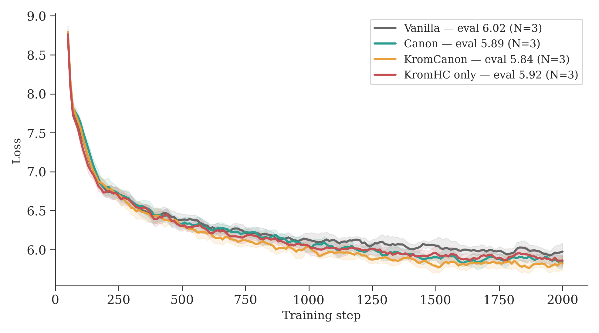
That’s what we found. We trained three GPT-21 variants from scratch on Apple Silicon, each adding one architectural idea on top of the previous:
- Vanilla, a standard GPT-2 baseline.
- Canon, which adds causal convolution layers before attention2, a recent technique from Allen-Zhu’s Physics of Language Models that gives each token a small window of local context before the global attention step.
- KromCanon, which takes Canon and adds KromHC3 multi-stream residual connections on top, replacing the single information highway with four parallel ones that are supposed to learn to share information.
Same data, same hyperparameters, same number of training steps. The only difference is architecture. A fourth variant, KromHC only (KromHC without Canon), isolates the contribution of each modification.
We wanted to see how each modification affects the model’s internal structure. What we stumbled onto instead is a question we did not find addressed in the KromHC paper: whether the mixing matrices actually learn to mix.
At our scale, they don’t. And a one-line initialization change revives them.
This post reports three findings. First, KromHC’s default initialization keeps the mixing matrices frozen near identity throughout training, a consequence of softmax gradient saturation. Second, a milder initialization revives nontrivial mixing. Third, once mixing is active, safety-contrast directions remain highly aligned across streams (cosine 0.994 ± 0.001, N=3), though different training runs discover unrelated directions. The downstream fine-tuning anomaly appears to correlate more with initial SFT loss than with mixing strength, though this boundary is approximate.
One stream, four streams
Modern transformers4 use a residual connection5 at every layer: \(x = x + F(x)\). All information flows through one stream per token. A recent line of work proposes splitting that single stream into multiple parallel ones that exchange information at every layer through learned mixing matrices6.
KromHC3 is one implementation. Four parallel streams replace the single residual stream. At each layer, a doubly stochastic mixing matrix \(H^{res}\) controls how much information flows between streams. The matrix is constrained so that no stream can grow unboundedly or collapse to zero.
In the reference implementation, every mixing weight is initialized to 0.03% swap, 99.97% identity. The four streams behave as independent copies of a single stream. This identity-like start is natural for optimization stability: the model begins as a standard transformer and is supposed to gradually discover useful mixing patterns. The KromHC reference implementation initializes b_res = [0, -8] and alpha_res = 0.01, and the Hyper-Connections paper6 uses the same near-identity principle.
The dial that can’t turn
In our bias=-8 runs, the dial never turns.
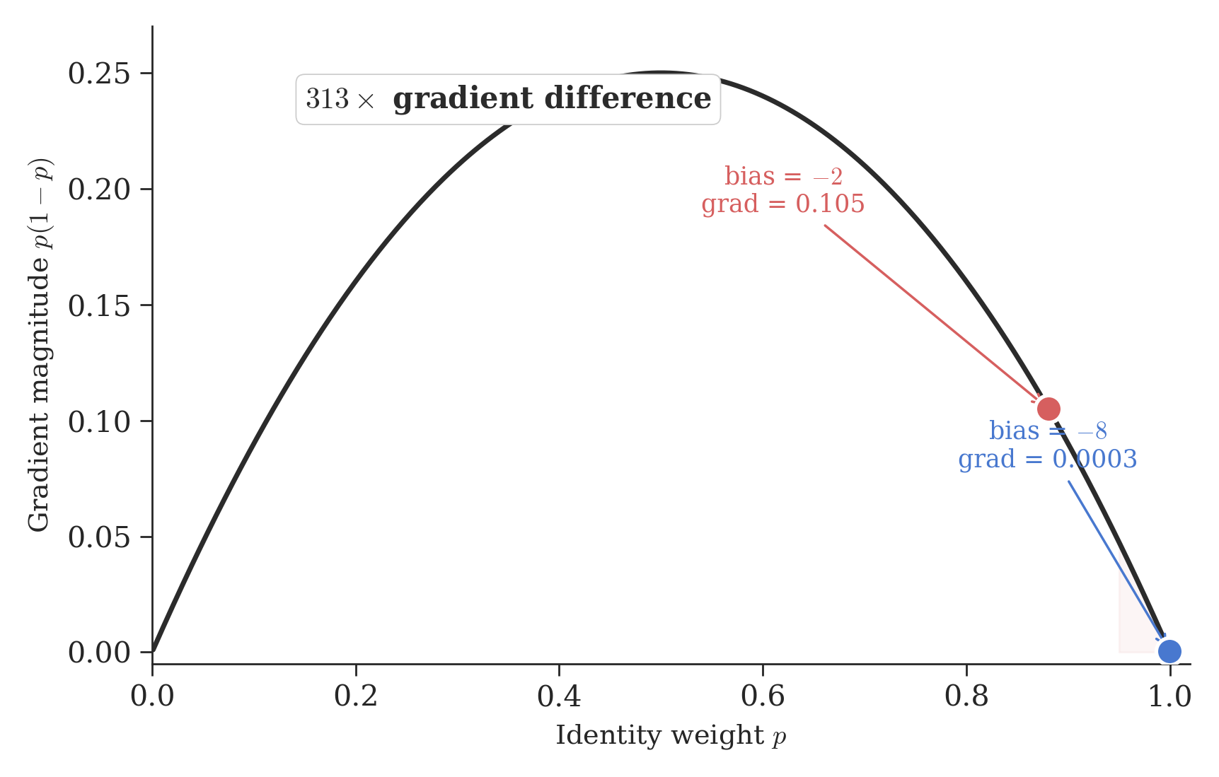
KromHC controls mixing through two pathways that feed into a softmax7 function. The first is a static bias, set to [0, -8] at initialization. The softmax converts this into two weights: an identity weight \(p\) (how much each stream keeps its own information) and its complement, the swap probability \(1-p\) (how much it exchanges with another stream). At a logit gap of 8, \(p = 0.9997\) and swap probability is \(0.03\%\), essentially zero. At our proposed gap of 2, \(p = 0.881\) and swap probability is \(12\%\). The second pathway is a dynamic component that modulates the mixing based on the input, controlled by a learned coefficient \(\alpha_{res}\).
The reason this matters is the softmax gradient. The gradient of a softmax output with respect to its input is \(p(1-p)\). At the default initialization (\(p = 0.9997\)), the gradient is \(0.9997 \times 0.0003 = 0.0003\). At our proposed initialization (\(p = 0.881\)), the gradient is \(0.881 \times 0.119 = 0.105\). That is a 313x difference.
In principle, the dynamic component could push the swap probability high enough for nontrivial mixing to emerge. In our bias=-8 runs, it doesn’t. The figure below shows the swap probability for every layer, at both initializations: the faint bar is what the static bias alone gives, and the solid bar is the best the model can achieve with dynamics on top.
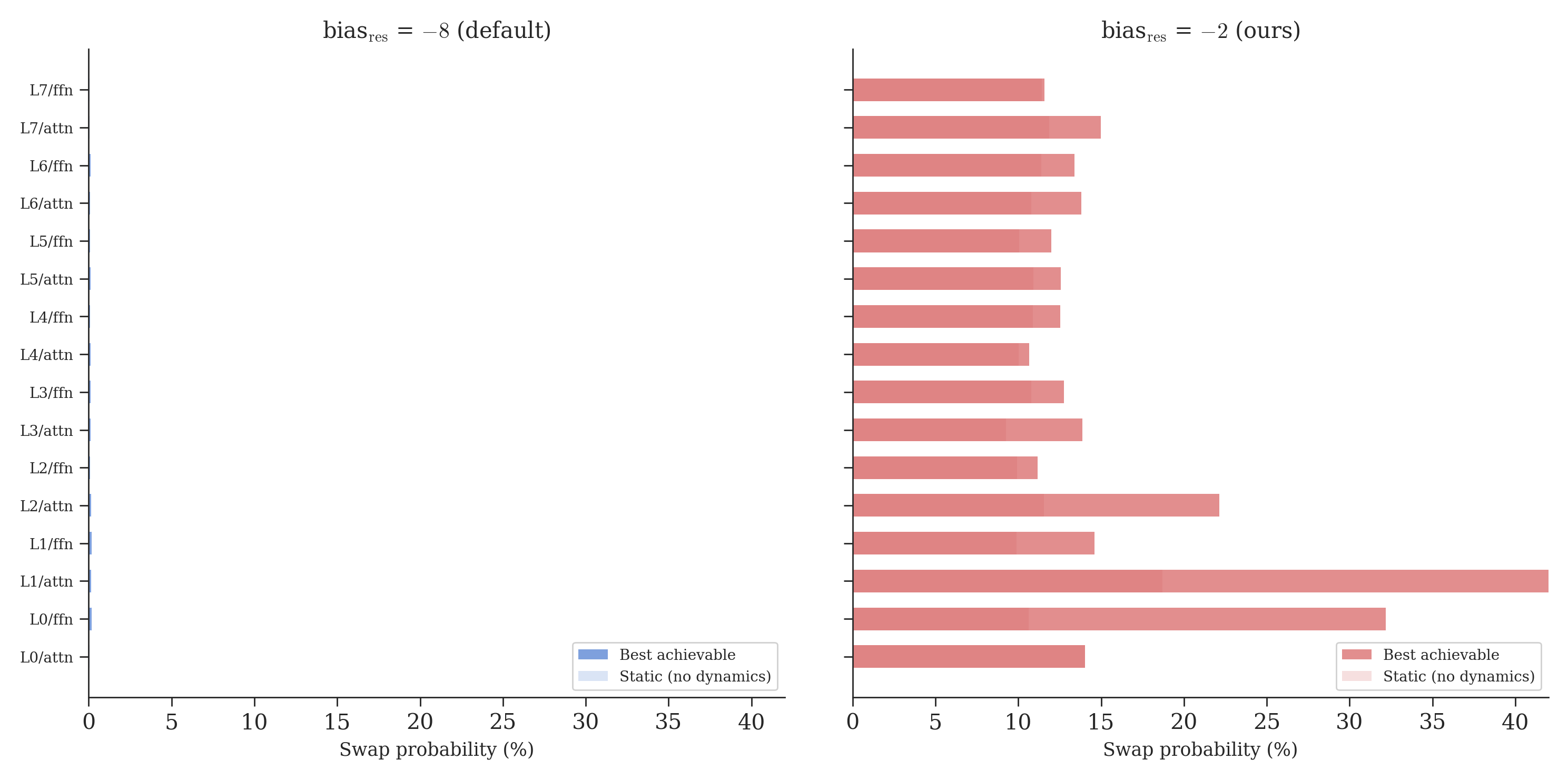
At bias=-8, the static swap probability is 0.03%. The model fights hard, pushing \(\alpha_{res}\) from 0.01 up to 0.92 in some layers. But even at maximum effort, the best achievable swap probability is about 0.4% (L2/attn). The model reaches for the dynamic lever and pulls it as hard as it can, but the static initialization is too deep. The steering wheel turns, but it’s not connected to the wheels.
At bias=-2, the static swap probability starts at 12%. Now the same dynamic component can push layers well beyond the identity regime. L0/ffn reaches 37% swap probability.
This is the gradient trap: initialize too deep in the saturated regime of a softmax, and the mixing path becomes effectively unlearnable.
Frozen vs alive
The contrast is even more striking when you look at the raw Kronecker factor weights8 that make up the mixing matrices. Each layer has two factors, each with an “identity weight” and a “swap weight.” At identity, all swap weights are zero. Any departure from zero means mixing is happening.
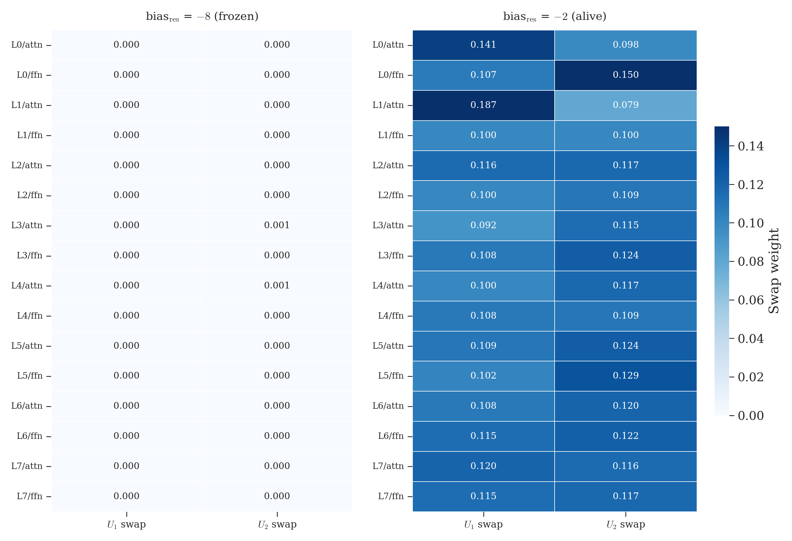
Left panel: blank white. Every single factor across all 16 layer/branch pairs stayed at its initialization value. Nothing moved. Right panel: variation everywhere. Some layers mix more (L0/attn: 0.129/0.129), others less (L1/ffn: 0.090/0.090), and the two factors within a layer can differ (L0/ffn: 0.100/0.148). The learned mixing becomes layer-specific. One glance tells you what the gradient trap does.
Layer-specific modulation under milder initialization
Once the initialization leaves the saturated regime, some layer-specific modulation emerges, but most of that topology is seed-dependent. The figure below shows the dynamic coefficient \(\alpha_{res}\) (how hard the model tries to modulate mixing) against the best achievable swap probability (whether it succeeds). Each dot is one layer/branch pair.
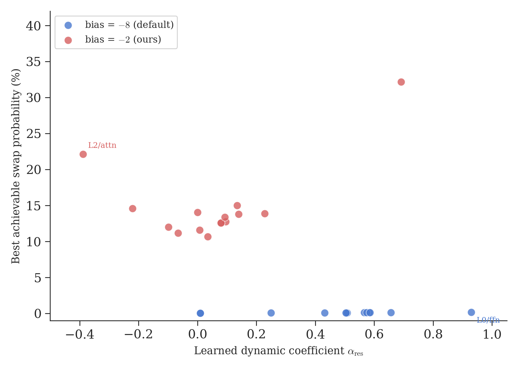
At bias=-8 (blue), every layer is trapped near 0% mixing. The model pushes \(\alpha_{res}\) as high as 0.93 (L2/attn), maximum effort, but the best achievable swap probability is still 0.4%. At bias=-2 (red), the same mechanism works: L0/ffn reaches \(\alpha = 0.84\) and achieves 37% swap probability. Some layers actively suppress mixing (L0/attn, L2/attn have negative \(\alpha\)), pulling their swap probability back down. The model builds a non-uniform topology: amplifying where mixing helps, suppressing where it doesn’t.
This pattern is stable from step 1000 to step 2000 within a single run. However, N=3 replication reveals that most of the topology is seed-dependent: only 5 of 16 layer/branch pairs maintain consistent \(\alpha_{res}\) sign across seeds. L0/ffn is the only layer that robustly reaches maximum amplification in all three runs. The non-uniform topology is real, but most of its details appear to be training-trajectory dependent rather than architecturally fixed. To our knowledge, nobody has visualized this for KromHC before.
Directions survive multi-stream coupling
The original motivation for this project was a question from interpretability research. Techniques like abliteration9 work by finding linear directions in a model’s internal representations that correspond to specific behaviors. Arditi et al. showed that “refusal is mediated by a single direction in the residual stream” and that removing it disables safety behavior. This works beautifully in standard single-stream transformers.
The worry with multi-stream architectures is intuitive: if a behavioral signal gets split across four rivers in four different orientations, the standard toolkit would break.
We tested this by fine-tuning all three variants on safety-contrast data (helpful vs harmful prompt pairs) and extracting the direction that separates them in each stream independently. An important caveat: at our loss level (perplexity10 around 330 to 400, not coherent text), the model cannot actually refuse anything. What we’re measuring is not a “refusal direction” but a safety-contrast direction, the geometric imprint that fine-tuning leaves on the representations. The direction is real. Whether it would control behavior in a converged model is a separate question we can’t answer at this scale.
With that caveat, the geometric finding is clean.
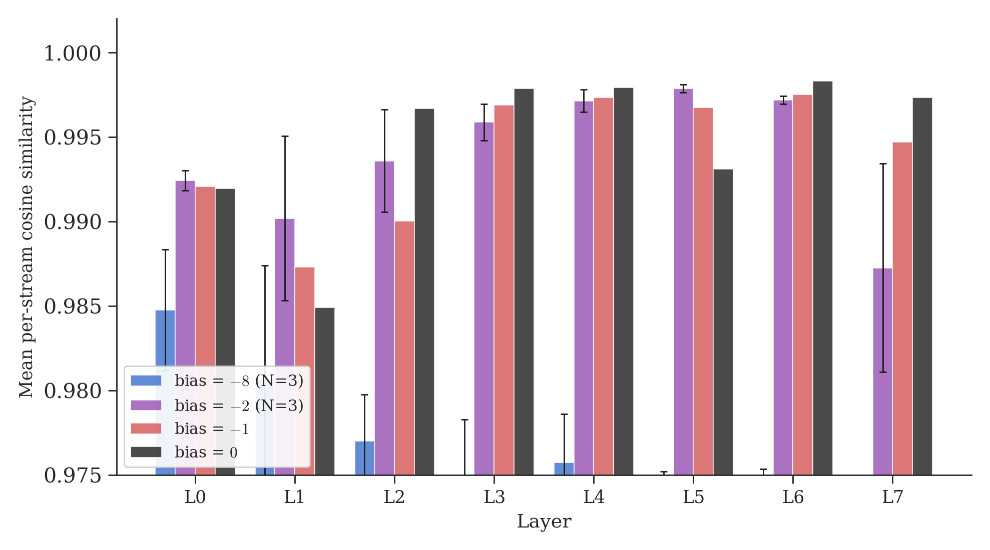
At bias=-8 (no mixing), per-stream cosines average 0.974 ± 0.005 across three seeds. In a 512-dimensional space, random directions would have cosine \(\approx 0 \pm 0.044\), so these are clearly not noise. Fine-tuning creates a consistent geometric signal across all streams. But small differences accumulate independently since the streams can’t talk to each other.
At our scale, the main effect appears thresholded rather than smoothly graded. Once mixing is turned on, cosines jump to a plateau: mean 0.994 ± 0.001 at bias=-2 (three seeds), 0.994 at bias=-1, 0.995 at bias=0. Every mixing configuration produces substantially higher cosines than the identity baseline, but the three mixing regimes are essentially indistinguishable from each other. A concurrent paper11 proves this theoretically: doubly stochastic mixing matrices12 contract inter-stream differences at every layer, with contraction factor \(|1-2s|\) where \(s\) is the swap probability. At bias=-2 (\(s = 0.12\)), the contraction factor is 0.76 per mixing operation. Over 8 layers with two operations each: \(0.76^{16} \approx 0.012\), meaning 98.8% of inter-stream difference is contracted away. At bias=-1 (\(s = 0.27\)), it is \(0.46^{16} \approx 0\), essentially perfect contraction. The plateau is expected: once mixing exceeds \(s \approx 0.1\), contraction saturates and additional mixing produces diminishing returns. Bias=0 (\(s = 0.5\), perfect contraction by construction) confirms this, producing the highest mean cosines in the sweep (0.995).
Multi-stream coupling doesn’t fragment representational directions. It homogenizes them. This holds even at n=8 streams (per-stream cosine 0.992 vs 0.994 at n=4, with identical eval loss). Whether this carries over to actual behavioral directions in a converged model is the natural next experiment.
An additional geometric observation: directions extracted from different architectures or different seeds are unrelated. Cross-architecture direction cosines (vanilla vs canon vs KromCanon) average |cos| ≈ 0.03 across N=3 seeds, indistinguishable from random in 512 dimensions. Cross-seed cosines within the same architecture are equally random. Each training run discovers its own safety-contrast direction, consistent with the non-identifiability results of Venkatesh and Kurapath13.
Safety fine-tuning and first-loss effects
In our initial seed, we observed what appeared to be a sharp phase transition: SFT loss increased at bias=-8 and bias=-2, but decreased at bias=-1 and bias=0. This suggested a functional threshold tied to mixing strength. Multi-seed replication (N=3) revealed a different pattern.
The SFT anomaly (loss increasing during fine-tuning) correlates with the pretrained model’s initial SFT loss, not with mixing strength. At bias=-8, one seed shows strong anomaly (first-loss 0.695, delta +0.253), one is flat (first-loss 0.752, delta +0.004), and one converges normally (first-loss 0.783, delta -0.175). The pattern is consistent with a first-loss threshold around 0.75: below it, models tend to overshoot during SFT; above it, they converge normally. But the boundary is approximate and the sample is small.
The geometric threshold remains robust. Per-stream cosines jump from 0.974 ± 0.005 (bias=-8, N=3) to 0.994 ± 0.001 (bias=-2, N=3) when mixing is turned on. Whether a separate functional threshold exists for downstream learning remains open.
Our current evidence supports a geometric threshold, not a functional one.
A gap in the literature
In the published KromHC paper, we found no visualization of the learned mixing weights, no measurement of how far they move from initialization, and no ablation isolating the mixing matrix from the routing matrices. The paper reports performance improvements and gradient norm trajectories, but does not directly address whether the mixing actually happens.
A natural counterargument: the KromHC dynamic coefficients are input-dependent, so the static initialization is just a starting point, and at larger scale the dynamic pathway might have sufficient signal to overcome it. We measured this directly (Section: The model sculpts its mixing). At our scale, the dynamic pathway tries (\(\alpha_{res}\) reaches 0.93) and appears unable to overcome the saturated initialization. The static initialization at \(-8\) places the system so deep in the saturated regime that the dynamic component cannot compensate. Whether this changes at 186M parameters and 454K steps is an open empirical question, but the mathematical structure of the saturation is scale-independent: \(p(1-p)\) at \(p = 0.9997\) is 0.0003 regardless of model size.
Compare this with DeepSeek’s mHC14, which uses a different parameterization called Sinkhorn-Knopp projection15 instead of softmax. Their approach doesn’t have the \(p(1-p)\) gradient bottleneck, because Sinkhorn-Knopp gradients flow through the projection operator rather than through a saturating nonlinearity. Whether their mixing matrices learn non-trivial patterns at scale is a question we cannot answer from the published results, but the parameterization itself does not have the structural barrier we identified.
Our claim is precisely scoped: at small scale (51M parameters) with the softmax parameterization and default initialization, multi-stream mixing does not meaningfully emerge. Whether it emerges at larger scale with the same parameterization remains unknown, because, to our knowledge, nobody has reported it.
What this means
This work sits at the intersection of mechanistic interpretability, training dynamics, and safety-relevant representation geometry. Our primary contribution is architectural: under the default softmax-based initialization at our scale, multi-stream mixing remains effectively frozen. The gradient trap, the routing vs mixing distinction, and the layer-specific modulation all concern parameter dynamics, not text quality, and hold at any loss level. The practical lesson: if you build a multi-stream model, do not assume the architecture you wrote is the architecture that trained. Inspect the learned mixing matrices. A model can have multi-stream equations on paper while behaving like redundant single-stream copies in practice.
The bias sweep reveals a symmetry. At one extreme (bias=-8), streams don’t mix: the architecture collapses to a single effective stream with four redundant copies. At the other extreme (bias=0), streams mix perfectly: the doubly stochastic contraction homogenizes representations, and the four streams converge to near-identical states11. Both extremes lose the benefit of multi-stream diversity. The useful regime lies between them, though across three seeds, eval loss does not clearly favor one initialization over another (5.836 ± 0.006 at bias=-8 vs 5.834 ± 0.004 at bias=-2). The downstream effects of mixing strength remain an open question.
If you’re building multi-stream architectures, monitor your mixing matrices during training. Log \(\|H^{res} - I\|\) at each checkpoint. If it stays near zero, your streams aren’t mixing. Consider a milder initialization (\(-2\) instead of \(-8\)), or switch to a parameterization that doesn’t saturate.
If you work on interpretability, our geometric finding suggests that multi-stream coupling preserves directional structure rather than fragmenting it. At our scale, a single direction extracted from any stream captures the same geometric signal. But we want to be clear: we tested whether the preconditions for abliteration hold under multi-stream coupling, not abliteration itself. Verifying the behavioral story requires a converged model, which is future work.
If you use KromHC, the architecture is more capable than its default initialization reveals. It has three independent channels of influence: routing, static mixing, and dynamic mixing. But the default configuration only activates the first. A one-line initialization change unlocks the other two.
Summary of results
Bias sweep (KromCanon, 8L512D)
All losses are eval loss (held-out split).
| Init bias | Swap prob | Gradient \(p(1-p)\) | Eval loss | Per-stream cosine | Seeds |
|---|---|---|---|---|---|
| \(-8\) | 0.03% | 0.0003 | 5.836 ± 0.006 | 0.974 ± 0.005 | 3 |
| \(-2\) | 12% | 0.105 | 5.834 ± 0.004 | 0.994 ± 0.001 | 3 |
| \(-1\) | 27% | 0.197 | 5.829 | 0.994 | 1 |
| \(0\) | 50% | 0.250 | 5.828 | 0.995 | 1 |
Architecture comparison (bias=-8, N=3)
| Architecture | Eval loss | Description |
|---|---|---|
| Vanilla | 6.016 ± 0.003 | Standard GPT-2 |
| Canon | 5.891 ± 0.003 | + causal convolution (ABCD) |
| KromCanon | 5.836 ± 0.006 | + Canon + KromHC (4 streams) |
The loss ordering KromCanon < Canon < Vanilla is consistent across all three seeds. Canon-ABCD (with Kaiming initialization and all four placement positions) accounts for most of the improvement over vanilla; KromHC adds a smaller further gain. Our FFN uses GELU rather than SwiGLU, so Canon-D placement may behave differently under gated activations.
What replicates
| Finding | Seeds | Robust? |
|---|---|---|
| Gradient trap (mixing frozen at bias=-8) | 3 | Yes |
| Per-stream cosine threshold (0.974 → 0.994) | 3 | Yes |
| Loss ordering (KromCanon < Canon < Vanilla) | 3 | Yes |
| Cross-seed directions at random baseline | 3 | Yes |
| SFT first-loss correlation (low first-loss → anomaly) | 3 | Approximate |
| Alpha topology (layer-specific mixing pattern) | 3 | Mostly seed-dependent |
Limitations and open questions
We want to be explicit about what this work does and does not establish:
- Robust (N=3). The gradient trap, per-stream cosine threshold (0.974 → 0.994), loss ordering (KromCanon < Canon < Vanilla), and cross-seed direction independence all replicate across three seeds.
- Approximate. The SFT anomaly correlates with initial SFT loss rather than mixing strength, but the boundary between anomalous and normal convergence is not perfectly sharp (1/3 seeds shows anomaly at bias=-8, vs 3/3 with the prior Canon-AB implementation). The alpha topology (which layers amplify vs suppress mixing) is mostly seed-dependent.
- Implementation note. Canon uses ABCD placement with Kaiming initialization and GELU activation. The original paper specifies SwiGLU; Canon-D placement may behave differently under gated activations.
- Scale. All experiments are at 51M parameters, 2000 training steps. The gradient trap is a property of the softmax parameterization and holds at any scale, but we have not verified whether mixing emerges at larger scale even with bias=-8 given more compute.
- Behavioral directions. We measure geometric properties (cosine similarity of per-stream directions), not behavioral effects. At our loss level (perplexity ~330-400), the model cannot refuse or comply. Whether the directional coherence we observe would translate to robust abliteration in a converged model is unknown.
All experiments on a single Apple M4 Pro, 24GB. Three GPT-2 variants at ~51M parameters, trained from scratch on FineWeb-Edu16. Code at github.com/teilomillet/kromcanon. I designed the experiments, chose the hypotheses, ran the bias sweep, caught the SFT anomaly, and pushed back on every overclaim. Claude drafted the text, wrote code, and ran searches. The experimental thinking was mine; the execution was collaborative.
GPT-2 is an older, well-understood language model architecture released by OpenAI in 2019. We use it as a baseline because its behavior is thoroughly studied, making it easy to isolate the effects of architectural changes. openai.com/research/better-language-models ↩︎
Canon layers are causal convolution layers from Allen-Zhu’s “Physics of Language Models, Part 4.1”. They add local token mixing before attention, improving reasoning depth with minimal parameter overhead (~0.5%). arxiv.org/abs/2512.17351 ↩︎
Wang et al., “KromHC: Kronecker-product Hyper-Connections”, 2025. It replaces standard residual connections with multi-stream mixing using Kronecker-factorized doubly stochastic matrices. arxiv.org/abs/2601.21579 ↩︎ ↩︎
Transformers are the architecture behind most modern AI language models (ChatGPT, Claude, Gemini, etc.). Introduced by Vaswani et al. in “Attention Is All You Need”, 2017. arxiv.org/abs/1706.03762 ↩︎
A residual connection is the
x = x + F(x)pattern. Instead of replacing the input with the output of a layer, you add the layer’s output to the input. This lets information flow directly through the network without being forced through every transformation, which makes deep networks much easier to train. Introduced by He et al., “Deep Residual Learning”, 2015. arxiv.org/abs/1512.03385 ↩︎Zhu et al., “Hyper-Connections”, 2024. The original proposal for multi-stream residual connections, where multiple parallel streams replace the single residual stream and mix at every layer. arxiv.org/abs/2409.19606 ↩︎ ↩︎
Softmax is a function that takes a list of raw numbers and converts them into probabilities that sum to 1. For example, softmax([2, 1]) gives roughly [0.73, 0.27]. It’s used everywhere in neural networks, from attention mechanisms to classification heads. ↩︎
Kronecker factors are the building blocks of KromHC’s mixing matrices. Instead of learning a full 4x4 mixing matrix (16 parameters), KromHC builds it as a Kronecker product of two 2x2 matrices (2 parameters each). Each 2x2 factor is a blend between “identity” (no mixing) and “swap” (exchange streams). The swap weight tells you how much mixing that factor contributes. ↩︎
Arditi et al., “Refusal in Language Models Is Mediated by a Single Direction”, 2024. They showed that safety-trained language models encode refusal behavior along a single linear direction in their internal representations, and that removing this direction disables refusal. arxiv.org/abs/2406.11717 ↩︎
Perplexity is the exponential of the loss. It roughly measures “how many words the model is confused between at each position.” A perplexity of 1 means the model always knows the next word. A perplexity of 400 means it’s choosing between about 400 equally likely options at every step. Modern production language models reach perplexities in the single digits. ↩︎
Liu, “The Homogeneity Trap: Spectral Collapse in Doubly-Stochastic Deep Networks”, 2026. This paper proves that doubly stochastic mixing suppresses representational diversity across streams, a phenomenon they call spectral collapse. arxiv.org/abs/2601.02080 ↩︎ ↩︎
A doubly stochastic matrix is a square matrix where every row sums to 1 and every column sums to 1. This constraint guarantees that the mixing is “fair”: no stream receives more total input than others, and no stream’s contribution is over- or under-weighted. It also guarantees that the total magnitude of the streams is preserved through the mixing. ↩︎
Venkatesh and Kurapath, “On the Non-Identifiability of Steering Vectors in Large Language Models”, 2026. Shows that steering vectors are fundamentally non-identifiable due to large equivalence classes of behaviorally indistinguishable interventions. arxiv.org/abs/2602.06801 ↩︎
Xie et al. (DeepSeek), “mHC: Manifold-Constrained Hyper-Connections”, 2025. Scales multi-stream residual connections using Sinkhorn-Knopp projection instead of softmax to enforce doubly stochastic mixing. arxiv.org/abs/2512.24880 ↩︎
Sinkhorn-Knopp projection is a method for turning any matrix into a doubly stochastic one by alternately normalizing rows and columns. Unlike softmax parameterization, the gradients flow through the projection operator and don’t suffer from the \(p(1-p)\) saturation problem. ↩︎
FineWeb-Edu is a large, high-quality dataset of educational web text curated by HuggingFace. We used it for pretraining because it provides clean, diverse text at scale. huggingface.co/datasets/HuggingFaceFW/fineweb-edu ↩︎