Abstract
Reinforcement learning from reasoning traces faces credit assignment at two levels: which problems deserve gradient (episode level) and which tokens within a solution contributed to success (token level). MaxRL (Tajwar et al., 2026) addresses the episode level by reweighting advantages by inverse success rate but treats every token in a successful rollout identically.
We propose a compositional credit assignment framework with a plug-compatible interface: any episode-level operator that depends only on group rewards composes with any token-level operator that depends only on per-position uncertainty, without either needing to know about the other. As one instantiation, we introduce SEPA (Selective Entropy Pooling with Annealing), a token-level variance reduction transform that pools execution-token surprisal while preserving planning-token surprisal.
Preliminary experiments (36 runs, ~159k generations) did not reach statistical significance. The predicted condition ranking appeared at a single early checkpoint but was not sustained in cumulative metrics, leaving open whether the effect is on learning speed or is simply noise at this scale. A mechanistic diagnostic on 318k tokens confirmed that SEPA reduces execution-token surprisal variance by 98% while leaving planning tokens unchanged (Figure 1). The contribution is twofold: a compositional framework that makes the independence between episode-level and token-level credit explicit, and SEPA as a concrete module within that framework, validated mechanistically but with underpowered training outcomes. We release all infrastructure to enable conclusive testing.
Introduction
Training language models to reason via reinforcement learning faces a credit assignment problem at two distinct levels.
At the episode level, the training signal must decide which problems deserve gradient. Standard RL algorithms such as GRPO (Shao et al., 2024) weight all problems by their reward variance regardless of difficulty. MaxRL (Tajwar et al., 2026) normalizes advantages by the success rate, giving hard problems gradient proportional to \(1/p\) and recovering the full maximum likelihood objective that standard RL truncates to first order.
At the token level, the signal must decide which tokens within a successful solution actually contributed to its success. MaxRL does not address this. Its gradient estimator averages uniformly over all tokens in successful trajectories:
\[\hat{g}_{\text{MaxRL}} = \frac{1}{K} \sum_{i: r_i=1} \nabla_\theta \log \pi_\theta(z_i \mid x)\]where \(K\) is the number of successes and \(\pi_\theta\) is the policy.1 In a 200-token reasoning trace, perhaps 5 tokens represent the actual insight: a strategy shift, an error correction, or a structural connection. The other 195 tokens are routine arithmetic. MaxRL treats them identically.
This paper makes two contributions:
- A compositional framework with a plug-compatible interface: episode-level operators depend only on group rewards, token-level operators depend only on per-position uncertainty (plus an optional structural mask), and any new module at either level composes with the rest of the stack without redefining it.
- SEPA, a variance reduction transform for the GTPO weighting signal that pools execution-token surprisal while preserving planning-token surprisal, validated mechanistically but with underpowered training outcomes.
We present preliminary experiments testing the framework in a factorial ablation on math reasoning. Our compute budget (~159k generations) was insufficient to distinguish the conditions at the observed effect sizes; we report power estimates for a conclusive test.
Background
Group Relative Policy Optimization. GRPO (Shao et al., 2024) generates \(N\) rollouts per prompt and uses group-relative advantages \(A_i = r_i - \bar{r}\). It weights all problems equally and applies the same scalar advantage to every token.
Maximum Likelihood RL. The ML objective decomposes as a harmonic sum over pass@\(k\) (Tajwar et al., 2026): \(\nabla J_{\text{ML}}(x) = \sum_{k=1}^{\infty} \frac{1}{k} \nabla \text{pass@}k(x)\). Standard RL keeps only \(k=1\). MaxRL recovers the full sum via
\[A_i^{\text{MaxRL}} = \frac{r_i - \bar{r}}{\bar{r} + \epsilon}\]For binary rewards with \(K\) successes out of \(N\) rollouts, correct completions receive advantage \((N-K)/K\) and incorrect completions receive \(-1\).
Entropy-Weighted Token Credit. GTPO (Tan et al., 2025) reshapes the scalar group advantage into per-token rewards using the policy’s own entropy. The formulation separates rollouts into correct (\(\mathcal{O}^+\)) and incorrect (\(\mathcal{O}^-\)) sets and defines a token-level reward \(\tilde{r}_{i,t} = \alpha_1 r_i + \alpha_2 \cdot (H_{i,t} / \sum_k H_{k,t}) \cdot d_t\), where \(H_{i,t}\) is the true policy entropy at position \(t\). Our implementation uses surprisal (the negative log-probability of the sampled token) as a cheaper proxy.
Process Reward Models. PRMs (Lightman et al., 2023); (Wang et al., 2023) score intermediate reasoning steps but require step-level annotations and a separate model. Our approach requires no annotations, using the model’s own surprisal as a proxy for decision importance.
Method: A Composable Credit Assignment Stack
We propose four independently toggleable layers, each addressing a different failure mode. Each layer is defined below in dependency order: later layers build on earlier ones.
| Layer | Level | What it decides | Failure mode addressed |
|---|---|---|---|
| MaxRL | Episode | Which problems get gradient | Easy problems dominate gradient |
| GTPO | Token | Which tokens get credit | All tokens weighted equally |
| HICRA | Token (structural) | Amplify planning tokens | No structural prior |
| SEPA | Token (surprisal) | Clean the uncertainty signal | Execution noise in surprisal |
Episode Level: MaxRL
Given \(N\) rollouts with binary rewards for a prompt, we compute episode-level advantages via the MaxRL formula above. When \(\bar{r} \leq \epsilon\) (no successes), all advantages are zero, because there is nothing to learn from a group where every rollout failed. Hard problems (small success rate \(\bar{r}\)) receive advantages scaled by \(1/\bar{r}\), recovering the maximum likelihood gradient.
Token Level: GTPO Surprisal Weighting
The episode-level advantage \(A_i\) is a scalar for the entire completion. To differentiate within the completion, we need a per-token signal. GTPO (Tan et al., 2025) treats tokens where the policy distribution spreads across many plausible continuations (high entropy) as decision points that receive amplified credit, and treats tokens where the next token was near-certain (low entropy) as routine.
Surprisal vs. entropy
A precise distinction is needed because our implementation departs from the original formulation. Tan et al. weight tokens by the true policy entropy, \(H(t) = -\sum_v p_\theta(v \mid \text{ctx}_t) \log p_\theta(v \mid \text{ctx}_t)\), which measures the spread of the model’s distribution over the full vocabulary at position \(t\). Computing this requires access to the full logit vector at each position. Surprisal is the information content of the single token actually sampled: \(S(t) = -\log p_\theta(t_{\text{sampled}} \mid \text{ctx}_t)\).
Surprisal is available directly from the sampling log-probabilities but is a noisier signal. The approximation breaks down in two directions. A token can have high surprisal but low entropy: if the model concentrates 95% of probability on one continuation and the sampler draws from the 5% tail, then the surprisal is high but the distribution was confident. Conversely, a token can have low surprisal but high entropy: if the model spreads probability uniformly across many continuations and the sampler happens to draw the mode, then the surprisal is low but the distribution was genuinely uncertain.
Surprisal adds a layer of noise on top of a problem that already exists with true entropy: execution tokens can have genuinely high distributional uncertainty for reasons unrelated to reasoning quality (e.g., the model spreading probability across equivalent phrasings of an arithmetic step). With true entropy, such tokens would still receive disproportionate GTPO credit. Surprisal makes this worse by introducing sampling artifacts (a peaked distribution can produce a high-surprisal outlier), but the core issue is that high uncertainty at execution tokens reflects procedural ambiguity, not strategic importance. SEPA addresses both sources of noise. Our generation pipeline stores only the sampled token’s log-probability, not the full logit vector, so we operate on the noisier signal.
Our implementation uses surprisal as the weighting signal.2 The GTPO weight at position \(t\) is
\[w(t) = \max\!\left(0,\; 1 + \beta\left(\frac{S(t)}{\bar{S}} - 1\right)\right), \qquad A^{\text{GTPO}}(t) = A_i \cdot w(t)\]where \(\bar{S}\) is the mean surprisal across the completion. Tokens with above-average surprisal receive amplified advantages; tokens with below-average surprisal receive dampened ones.
Canonical GTPO vs. our implementation
| Aspect | Canonical GTPO | Our implementation |
|---|---|---|
| Signal | True entropy \(H(t) = -\sum_v p \log p\) | Surprisal \(S(t) = -\log p(t_{\text{sampled}})\) |
| Partition | Separate \(\mathcal{O}^+\)/\(\mathcal{O}^-\); inverse-\(H\) for \(\mathcal{O}^-\) | Unified; advantage sign for directionality |
| Shaping | Additive: \(\tilde{r} = \alpha_1 r + \alpha_2 \frac{H}{\sum H} d_t\) | Multiplicative: \(A(t) = A_i \cdot w(t)\) |
| Normalization | Sum over sequences at position \(t\) | Mean over all tokens; clamped \(\geq 0\) |
Planning Token Identification and HICRA
Both HICRA and SEPA require identifying which tokens correspond to planning (high-level strategic reasoning) vs. execution (routine procedural steps). This distinction is grounded in the two-phase learning dynamics reported by Wang et al. (2025): RL training first consolidates procedural reliability (execution-token entropy drops sharply), then shifts to exploration of strategic planning (semantic diversity of planning tokens increases). Once procedural skills are mastered, the bottleneck for improved reasoning is strategic exploration.
Strategic Gram detection. Wang et al. introduce Strategic Grams (SGs) as a functional proxy for planning tokens: \(n\)-grams (\(n \in [3,5]\)) that function as semantic units guiding logical flow (deduction, branching, and backtracing). Their pipeline identifies SGs via (1) semantic clustering of \(n\)-grams using sentence embeddings, (2) corpus-level frequency analysis (Cluster Document Frequency), and (3) filtering for the top 20% most frequent clusters. Our implementation uses a simplified variant: a curated list of 18 strategic phrases matched via word-boundary regex over sliding token windows.3 This produces a binary mask \(\mathbf{1}_{\text{plan}}(t) \in \{0, 1\}\) for each token.
The planning mask as a swappable component. The planning mask is the foundation on which both HICRA and SEPA stand. If the mask misidentifies tokens, then both methods operate on corrupted signal. The framework is designed so that the mask is a swappable module: any classifier that produces a binary planning/execution partition over tokens (learned, attention-based, or the full SG pipeline) can be substituted without changing anything else in the stack.
HICRA advantage. Given the planning mask, HICRA (Wang et al., 2025) amplifies planning-token advantages after GTPO weighting:
\[A^{\text{HICRA}}(t) = A^{\text{GTPO}}(t) + \alpha \cdot |A^{\text{GTPO}}(t)| \cdot \mathbf{1}_{\text{plan}}(t)\]For positive advantages, planning tokens are amplified by factor \((1+\alpha)\); for negative advantages, the penalty is reduced by factor \((1-\alpha)\). The sign is never flipped. Wang et al. report consistent improvements of 2–6 points on math benchmarks across multiple model families.
SEPA: Selective Entropy Pooling with Annealing
SEPA uses the same planning mask as HICRA but operates at a different point in the pipeline with a different mechanism. Where HICRA acts after GTPO weighting to boost planning advantages, SEPA acts before GTPO weighting to clean the surprisal signal that GTPO consumes.
Entropy-weighted credit assignment is noisy in the execution region regardless of how entropy is measured. Execution tokens typically have low uncertainty (predictable continuations), but some execution tokens have genuinely high uncertainty for reasons unrelated to reasoning quality: the model choosing between two equivalent phrasings of an arithmetic step, for instance. These tokens receive disproportionate GTPO amplification even though the choice does not affect solution correctness. Using surprisal rather than true entropy makes this worse, but the core problem is that high uncertainty at execution tokens reflects procedural ambiguity, not strategic importance.
SEPA leaves planning tokens alone and compresses execution tokens toward their group mean. Given the execution set \(\mathcal{E} = \{t : \mathbf{1}_{\text{plan}}(t) = 0\}\) and its mean surprisal \(\bar{S}_{\mathcal{E}}\):
\[S^{\text{SEPA}}(t) = \begin{cases} S(t) & \text{if } \mathbf{1}_{\text{plan}}(t) = 1 \quad \text{(planning: unchanged)} \\ \lambda \cdot \bar{S}_{\mathcal{E}} + (1-\lambda) \cdot S(t) & \text{otherwise} \quad \text{(execution: pooled)} \end{cases}\]where \(\lambda \in [0,1]\) is the pooling strength.
Worked example
Consider a 10-token completion where tokens 3 and 7 are planning tokens:
| Token | 1 | 2 | 3 | 4 | 5 | 6 | 7 | 8 | 9 | 10 |
|---|---|---|---|---|---|---|---|---|---|---|
| Role | exec | exec | plan | exec | exec | exec | plan | exec | exec | exec |
| \(S(t)\) | 0.2 | 0.3 | 1.8 | 0.1 | 0.9 | 0.2 | 2.1 | 0.3 | 0.1 | 0.2 |
Token 5 is an execution token with surprisal 0.9, perhaps because the model chose between two equivalent ways to write a subtraction. Without SEPA, GTPO amplifies token 5 nearly as much as the planning tokens at positions 3 and 7.
With SEPA at \(\lambda=1\), all eight execution-token surprisals are replaced by their mean \(\bar{S}_{\mathcal{E}} \approx 0.29\). Token 5 drops from 0.9 to 0.29; tokens 3 and 7 remain at 1.8 and 2.1. When GTPO then weights by \(S(t)/\bar{S}\), planning tokens dominate the weighting.
Training schedule
Applying full pooling (\(\lambda=1\)) from the start would modify the surprisal distribution before the model has established a stable baseline. We anneal \(\lambda\) linearly from 0 to 1 over the course of training, with an optional delay of \(d\) steps (no pooling during the delay) so the model first establishes a baseline distribution. A correctness gate prevents SEPA from activating until the model reaches a minimum solve rate; once the gate opens, it stays open permanently to avoid oscillation.4 In our experiments we used the linear schedule with \(d=10\) and a correctness gate at 10%.
Execution variance as a phase transition signal
The linear schedule assumes the transition from procedural consolidation to strategic exploration happens proportionally to training steps. This assumption is crude: the transition depends on the model, the task, and the data, not the wall clock. A more principled alternative is to let the model’s own behavior determine when to intervene. Wang et al. (2025) describe two learning phases (procedural consolidation, then strategic exploration) but observe the transition post hoc. Execution-token surprisal variance provides a direct readout of this transition: when the model has mastered routine procedures, execution-token surprisal concentrates (variance drops), and the remaining variance lives in planning tokens. An adaptive schedule that ties \(\lambda\) to execution variance would detect this transition automatically, increasing pooling strength when the model’s behavior indicates that procedures are stable, without requiring a hand-tuned step count. This means SEPA could generalize across tasks and model sizes without re-tuning the schedule, because the trigger is intrinsic to the learning dynamics rather than extrinsic to the training clock. We implemented such a schedule (using an exponential moving average of execution variance), but at our training length the variance signal was too noisy to evaluate it.
SEPA and HICRA: complementary, not competing
Both use the planning mask \(\mathbf{1}_{\text{plan}}\), but they operate at different points in the pipeline with different mechanisms. SEPA operates before GTPO: it reduces execution surprisal variance so that GTPO weighting is less noisy (noise reduction). HICRA operates after GTPO: it amplifies the already-weighted planning advantages (signal amplification). These are complementary: SEPA cleans the input to GTPO, and HICRA boosts the output. The full composition would be SEPA → GTPO → HICRA, applying noise reduction and signal amplification simultaneously. Our current implementation supports only one or the other per run; in our experiments, each condition used HICRA or SEPA, not both. Testing the full three-stage composition is a natural next step.
Instantaneous Independence, Dynamic Coupling
The two levels compose by sequential application: MaxRL produces the episode advantage \(A_i\), then SEPA+GTPO distribute it across tokens. The final token-level advantage factorizes as
\[A^{\text{full}}(t) = A_i^{\text{MaxRL}} \cdot w^{\text{SEPA}}(t)\]At any single training step, the two factors are computed from disjoint inputs:
- \(A_i^{\text{MaxRL}}\) depends on rewards only (the group success rate).
- \(w^{\text{SEPA}}(t)\) depends on token surprisal only (the model’s per-position uncertainty), given a fixed \(\lambda_t\).
Neither reads the other’s output. The factorization is exact, not approximate; the two transforms are instantaneously independent once \(\lambda_t\) is determined.
One qualification: SEPA’s correctness gate sets \(\lambda_t = 0\) until the model’s solve rate exceeds a threshold, which means \(\lambda_t\) depends on reward history during the startup phase. Once the gate opens (permanently), \(\lambda_t\) follows a deterministic schedule that depends only on the step count (linear) or execution-token variance (adaptive), neither of which reads the current step’s rewards. The independence claim holds strictly after gate opening; before that, the token-level operator is trivially inactive (\(\lambda_t = 0\), so \(w(t) = 1\) for all \(t\)).
The interface contract
The value of this factorization is not the multiplication itself but the constraint it imposes on module design.
Definition 1 (Composable credit assignment). An episode-level operator \(f\) is any function \(f: \mathcal{R}^N \to \mathbb{R}^N\) that maps group rewards to per-completion advantages, depending only on the reward vector \((r_1, \ldots, r_N)\). A token-level operator \(g\) is any function \(g: \mathbb{R}^T \times \{0,1\}^T \to \mathbb{R}^T_{\geq 0}\) that maps per-position uncertainty signals and an optional structural mask to non-negative token weights, depending only on the model’s per-position distribution (entropy, surprisal, or attention) and the mask. The two operators compose by multiplication: \(A^{\text{full}}(t) = f(\mathbf{r})_i \cdot g(\mathbf{s}, \mathbf{m})_t\). Because \(f\) reads only rewards and \(g\) reads only per-position signals, any new module at either level composes with the rest of the stack without modification.
This means that replacing MaxRL with a different episode-level selector, or replacing SEPA with a different surprisal transform, requires no changes to the other level. The contract turns the factorization from a mathematical observation into a design principle for building and ablating credit assignment components independently.
Across training steps, the two levels are dynamically coupled through the shared model parameters \(\theta\). Token-level credit assignment (SEPA) changes which behaviors are reinforced, which changes the model, which changes future success rates, which changes MaxRL’s episode-level reweighting. Conversely, MaxRL’s problem reweighting changes which problems the model improves on, which changes the surprisal distribution that SEPA operates on. This is the standard structure of modular systems with shared state: no direct coupling at each step, but indirect coupling through state that evolves over time.
Algorithm: one training step
The complete pipeline for one training step, making explicit the order of operations and the inputs each module consumes. Our experiments tested SEPA or HICRA per condition, never both simultaneously; the three-stage combination (SEPA → GTPO → HICRA) is untested.
\[ \begin{aligned} &\textbf{Input: } \text{prompt } x, \text{ rollouts } \{z_1, \ldots, z_N\} \text{ with rewards } \{r_1, \ldots, r_N\} \\ &\qquad\quad \text{per-token log-probs } \ell_{i,t} \\ &\qquad\quad \text{schedule parameters: } \lambda_t, \beta, \alpha \\[8pt] &\textit{// Episode-level: depends only on rewards} \\ &\bar{r} \leftarrow \operatorname{mean}(r_1, \ldots, r_N) \\ &\textbf{if } \text{MaxRL}\textbf{:} \\ &\qquad A_i \leftarrow (r_i - \bar{r}) \,/\, (\bar{r} + \varepsilon) \quad \text{for each } i \\ &\textbf{else:} \\ &\qquad A_i \leftarrow r_i - \bar{r} \quad \text{for each } i \quad \text{(GRPO)} \\[8pt] &\textit{// Token-level: depends only on per-position uncertainty + mask} \\ &\textbf{for each } \text{rollout } i\textbf{:} \\ &\qquad S_{i,t} \leftarrow -\ell_{i,t} \quad \text{for each token } t \quad \text{(surprisal)} \\ &\qquad m_t \leftarrow \operatorname{DetectPlanning}(z_i) \quad \text{(strategic gram mask)} \\[6pt] &\qquad \textit{// SEPA: pool execution surprisal (before GTPO)} \\ &\qquad E \leftarrow \{t : m_t = 0\} \\ &\qquad \bar{S}_E \leftarrow \operatorname{mean}(\{S_{i,t} : t \in E\}) \\ &\qquad \textbf{for each } t \in E\textbf{:} \\ &\qquad\qquad S_{i,t} \leftarrow \lambda_t \cdot \bar{S}_E + (1 - \lambda_t) \cdot S_{i,t} \\[6pt] &\qquad \textit{// GTPO: weight by (cleaned) surprisal} \\ &\qquad \bar{S}_i \leftarrow \operatorname{mean}(\{S_{i,t}\}) \\ &\qquad \textbf{for each } t\textbf{:} \\ &\qquad\qquad w_t \leftarrow \max(0,\; 1 + \beta \cdot (S_{i,t} / \bar{S}_i - 1)) \\ &\qquad\qquad A_{i,t} \leftarrow A_i \cdot w_t \\[6pt] &\qquad \textit{// Optional HICRA: amplify planning advantages (after GTPO)} \\ &\qquad \textbf{for each } t \text{ where } m_t = 1\textbf{:} \\ &\qquad\qquad A_{i,t} \leftarrow A_{i,t} + \alpha \cdot |A_{i,t}| \\[8pt] &\textit{// Policy gradient update} \\ &\hat{g} \leftarrow \sum_{i,t} A_{i,t} \cdot \nabla_\theta \log \pi_\theta(z_{i,t} \mid z_{i,<t}, x) \\ &\theta \leftarrow \theta - \eta \cdot \hat{g} \end{aligned} \]Experiments
Design
We tested the framework in a factorial ablation crossing episode-level advantage (GRPO, MaxRL) with token-level transform (none, GTPO+HICRA, GTPO+SEPA), yielding 5 conditions:
| ID | Episode-level | Token-level | Purpose |
|---|---|---|---|
| C1 | GRPO | None (flat) | Baseline |
| C3 | GRPO | GTPO+HICRA | Token-level comparator |
| C4 | GRPO | GTPO+SEPA | Core claim (SEPA) |
| C5 | MaxRL | None (flat) | Episode-level replication |
| C8 | MaxRL | GTPO+SEPA | Episode + token (tested) |
Setup. Qwen3-4B-Instruct-2507 fine-tuned with LoRA (rank 64) on math reasoning with binary correctness reward. 16 problems per step, 16 rollouts per problem (256 generations/step), temperature 0.7, max 2048 tokens. AdamW with lr = 5 × 10⁻⁵. GTPO β = 0.1, HICRA α = 0.2, SEPA annealing over 100 steps with 10-step delay.
Budget. Due to compute constraints, we ran two campaigns:
- Pilot: all 8 conditions (including C2, C6, and C7) × 2 seeds × 20 steps = 16 runs.
- Lean: 5 conditions × 4 seeds × 12–16 steps (truncated by budget) = 20 runs.
Total: 36 runs, ~622 training steps, and ~159k generations.
Results
No significant separation
All conditions clustered within ±2 percentage points of each other throughout training. At step 10 of the lean campaign (the latest step where all 20 runs had data), correctness rates ranged from 32.9% to 35.1%.
| Condition | Correct rate | Std |
|---|---|---|
| C1: GRPO + none | 32.9% | ±2.1% |
| C3: GRPO + GTPO+HICRA | 33.2% | ±1.0% |
| C4: GRPO + GTPO+SEPA | 33.4% | ±0.7% |
| C5: MaxRL + none | 34.5% | ±1.3% |
| C8: MaxRL + GTPO+SEPA | 35.1% | ±1.0% |
Directional trends (point estimates)
The ordering at step 10 matched the predicted ranking: C8 (MaxRL+SEPA) > C5 (MaxRL alone) > C4 (SEPA alone) > C3 (HICRA) > C1 (baseline), though no pairwise difference was statistically significant. In the pilot campaign (step 19, 2 seeds), conditions converged to ~50% and the ordering dissolved.
Area under the learning curve
If the effect is on learning speed rather than final accuracy, then the right metric is cumulative sample efficiency: the area under the correctness curve (AUC). We computed trapezoidal AUC per run over two windows and report bootstrap 95% confidence intervals on the normalized AUC (mean correctness rate averaged over the training window).
| Condition | Steps 0–10 | Steps 0–15 |
|---|---|---|
| C1: GRPO + none | 43.9% [43.8, 44.1] | 41.4% [41.3, 41.6] |
| C3: GRPO + GTPO+HICRA | 44.1% [43.8, 44.5] | 41.8% [41.5, 42.1] |
| C4: GRPO + GTPO+SEPA | 44.0% [43.7, 44.2] | 41.8% [41.6, 42.0] |
| C5: MaxRL + none | 44.2% [43.8, 44.6] | 41.6% [41.4, 42.0] |
| C8: MaxRL + GTPO+SEPA | 44.0% [43.6, 44.4] | 41.2% [40.8, 41.6] |
With a 10-step delay and a 100-step linear ramp, \(\lambda\) reached only 0.05 at step 15 and never exceeded 0.10 across all experiments; SEPA operated at less than 10% of its designed strength throughout. These experiments test whether SEPA produces a detectable signal at less than 10% of its designed operating strength; they do not test the method at its intended configuration.
The AUC analysis showed smaller differences than the step-10 snapshot: all conditions fell within a 0.3pp band at steps 0–10 and a 0.6pp band at steps 0–15, with overlapping confidence intervals. No pairwise delta excluded zero at steps 0–10. At steps 0–15, GRPO+SEPA (C4) showed a marginally significant advantage over baseline (+0.4pp, 95% CI [0.1, 0.6]), but this is a single comparison among many. The predicted ranking (C8 first) did not appear in AUC terms.
Mechanistic diagnostic: does SEPA reshape the surprisal distribution?
Independent of the correctness signal, we verified directly that SEPA operates as designed. We extracted per-token surprisal values from 2,560 generations (16 seeds × 20 steps × 8 generations/step; 318k tokens total) logged during a prior MaxRL+SEPA campaign, reconstructed the planning mask via strategic gram detection, and compared the raw surprisal distribution (\(\lambda=0\)) against the pooled distribution (\(\lambda=1\)). The mask labeled 9,899 of 318,225 tokens (3.1%) as planning, with at least one planning phrase detected in 1,655 of 2,560 generations (65%). The low planning ratio is consistent with the expected structure of math reasoning traces, where most tokens are routine computation.
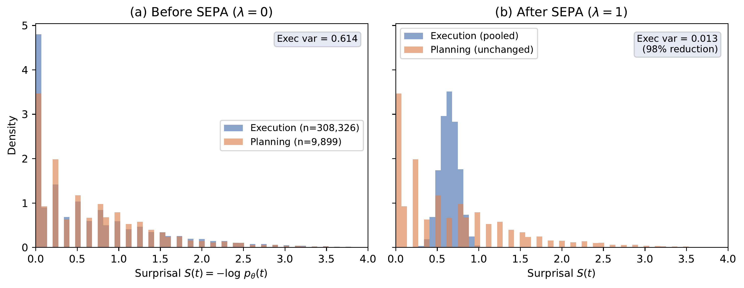
Surprisal distributions before and after SEPA pooling (318k tokens, 16 seeds). (a) Before: execution (blue) and planning (orange) tokens overlap broadly. High-surprisal execution tokens receive disproportionate GTPO amplification. (b) After (λ=1): execution tokens collapse to their mean (variance 0.614 → 0.013, 98% reduction). Planning tokens are unchanged. GTPO weighting now concentrates credit on planning tokens.
Before pooling, execution and planning tokens had nearly identical surprisal distributions (means 0.645 and 0.677), with execution variance 0.614. After pooling, execution-token variance dropped to 0.013: a 98% reduction. Planning tokens were unchanged. The execution distribution collapsed to a narrow spike around the execution mean; the planning distribution retained its original spread across [0, 4].
This confirms the mechanism: SEPA reduces execution-token surprisal variance so that GTPO weighting concentrates credit on planning tokens. The open question is whether this downstream concentration produces a measurable training signal at the effect sizes and training lengths we tested.
Power analysis
Prior paired experiments estimated an effect size of ~0.2 percentage points for the SEPA/HICRA comparison, requiring ~23k generations per arm for 80% power. Our lean campaign provided ~5k generations per condition at step 10. A conclusive test of the token-level hypothesis would require roughly 4–5× our current budget.
Discussion
Credit assignment may affect speed, not ceiling. The step-10 snapshot showed the predicted ranking (C8 > C5 > C4 > C3 > C1), but the AUC analysis revealed this to be an artifact of measuring at a single point: integrated over the training curve, all conditions fell within a 0.3pp band with overlapping confidence intervals.
This does not rule out a speed effect; it means our runs were too short to detect one via AUC. If the stack helps models learn faster rather than learn better, then the effect would appear as a wider AUC gap in early training that closes as conditions converge. With only 10–15 steps of usable data and \(\lambda\) never exceeding 0.10 (pilot) or 0.06 (lean), the mechanism reached less than a tenth of its designed strength. A meaningful AUC comparison requires runs long enough for the early-training advantage to accumulate before convergence erases it.
Token-level credit assignment methods are typically evaluated by final performance after a fixed training budget. If the benefit is faster convergence, then methods that appear equivalent at convergence may differ substantially in sample efficiency, and the right metric is area under the learning curve, not a point estimate.
What we planned vs. what we found. We began with the hypothesis that SEPA would produce a measurable correctness improvement over HICRA and that composing it with MaxRL would yield the best overall condition. We designed a 2 × 4 factorial ablation with five hypotheses, eight conditions, and a target budget of 64 runs at 100 steps each (~1.6M generations).
The experiment evolved in three phases. First, a pilot (16 runs, 20 steps) validated that all conditions ran correctly but showed no separation: every cell landed within ±2% of every other. Second, we cut the design from 8 conditions to 5 and from 8 seeds to 4 to reduce compute. Third, the lean campaign was terminated at step 12–16 when compute budget was exhausted.
At that point we had ~159k of the planned 1.6M generations. The original hypothesis was not supported, nor was it refuted. What emerged instead was the ranking in early training that dissolved as conditions converged. This shifted the paper from a claim that SEPA improves correctness to a composable framework with preliminary evidence that credit assignment may affect learning speed.
We report this trajectory because the reframing was forced by the data, not constructed after the fact. The original hypotheses remain testable with more compute; the speed hypothesis is new and was not anticipated by the original design.
The framework contribution stands independent of the empirical result. The composable stack (separating episode-level from token-level, and within token-level separating surprisal cleaning from advantage boosting) is a useful abstraction regardless of whether SEPA ultimately outperforms HICRA. It enables systematic ablation of credit assignment components and clarifies what each mechanism does.
Why the signal may be small. The most likely explanation is training length. Our runs reached 12–20 steps of a 100-step annealing schedule (with a 10-step delay), so \(\lambda\) never exceeded 0.10. Model capacity may also matter: at 4B parameters with rank-64 LoRA, the model may learn to reason well enough that advantage computation details are secondary to raw problem exposure. The task itself may be a factor: math problems with binary reward may not produce enough variation in planning-token surprisal for surprisal-based methods to differentiate themselves.
What would be needed. A conclusive version of this experiment would require:
- ~8 seeds per condition (vs. 4).
- ~100 steps per run (to let SEPA fully anneal).
- A larger model or harder task to increase the room for credit assignment to matter.
- Logging per-token surprisal distributions to test the mechanistic hypothesis directly.
- Logging full logit vectors for at least one run to decompose execution-token variance into genuine distributional entropy and sampling noise, directly resolving how much of the variance SEPA removes is an artifact of the surprisal approximation vs. a real property of the policy.
We estimate this at ~800k–1M generations total, roughly 5–6× our current budget.
Automatic phase detection. The adaptive \(\lambda\) schedule connects to a broader observation: SEPA does not just clean the surprisal signal; it provides a readout of training phase via execution-token variance. When execution variance is high, the model has not yet consolidated procedures, and pooling would distort a still-evolving distribution. When execution variance drops, procedural skills are stable, and the remaining surprisal variation lives in planning tokens. The adaptive schedule closes the loop by using this readout to control the intervention, replacing an extrinsic step count with an intrinsic behavioral signal. At our training length, the variance estimate (via exponential moving average) was too noisy to evaluate this schedule. Testing whether it outperforms linear annealing, and whether it generalizes across tasks without re-tuning, requires the longer runs described above.
Limitations
- Planning mask quality. Our regex-based strategic gram detector (18 hand-curated phrases) is simpler than the full semantic clustering pipeline (Wang et al., 2025) and has not been validated against human annotations. The failure modes are asymmetric, and this asymmetry points directly at the highest-value improvement. False negatives (planning tokens mislabeled as execution) are actively destructive: SEPA pools away their surprisal signal, inverting the intended effect. False positives (execution tokens mislabeled as planning) are benign: SEPA simply leaves their noise unchanged. This means the mask’s recall on planning tokens matters more than its precision, and the first priority for improving the stack is reducing false negatives. The mask also misses implicit planning: a model may shift strategy mid-sequence without producing any of the 18 trigger phrases. A learned or attention-based detector that captures implicit planning would address both failure modes. We designed the mask as a swappable component specifically to enable this upgrade.
- Surprisal vs. entropy. Our GTPO implementation uses surprisal (\(-\log p\) of the sampled token) rather than the true policy entropy that the original formulation specifies (Tan et al., 2025), and does not separate rollouts into correct/incorrect sets. Surprisal compounds a problem that exists even with true entropy (high-uncertainty execution tokens receiving disproportionate credit) by adding sampling artifacts from peaked distributions.
- Insufficient compute. Our primary results are not statistically significant. We report them as directional evidence, not conclusions.
- Single model and task. Qwen3-4B on math reasoning only.
- Truncated runs. The original design called for 100 steps per run; we reduced to 40 for the lean campaign and then cut short at step 12–16 because of compute budget exhaustion.
Conclusion
We proposed a composable framework for credit assignment in RL for reasoning that separates two complementary levels: episode-level objective selection (MaxRL) and token-level credit distribution (SEPA+GTPO). The framework provides a systematic way to ablate credit assignment components and understand what each contributes.
We introduced SEPA, which reduces execution-token surprisal variance before surprisal-based weighting. A mechanistic diagnostic confirmed that SEPA reduces execution variance by 98% while leaving planning tokens unchanged. The theoretical argument for the composition is that MaxRL decides which problems get gradient and SEPA+GTPO decides which tokens get credit; neither interferes with the other. Beyond variance reduction, execution-token surprisal variance may serve as an intrinsic signal for detecting the procedural-to-strategic phase transition, enabling an adaptive schedule that requires no hand-tuned step count; this is architecturally supported but untested at our training scale.
Our experiments showed that C8 (MaxRL+SEPA) ranked first at a single early checkpoint, though this ordering did not persist in cumulative metrics and did not reach statistical significance at the scale tested. A conclusive test requires approximately 5× more compute. We release the framework and experimental infrastructure to enable that test.
References
- Lightman, H., Kosaraju, V., Burda, Y., Edwards, H., Baker, B., Lee, T., Leike, J., Schulman, J., Sutskever, I., & Cobbe, K. (2023). Let’s Verify Step by Step. arXiv:2305.20050.
- Shao, Z., Wang, P., Zhu, Q., Xu, R., Song, J., Bi, X., Zhang, H., Zhang, M., Li, Y. K., Wu, Y., & Guo, D. (2024). DeepSeekMath: Pushing the Limits of Mathematical Reasoning in Open Language Models. arXiv:2402.03300.
- Tajwar, F., Zeng, G., Zhou, Y., Song, Y., Arora, D., Jiang, Y., Schneider, J., Salakhutdinov, R., Feng, H., & Zanette, A. (2026). Maximum Likelihood Reinforcement Learning. arXiv:2602.02710.
- Tan, H., Wang, Z., Pan, J., Lin, J., Wang, H., Wu, Y., Chen, T., Zheng, Z., Tang, Z., & Yang, H. (2025). GTPO and GRPO-S: Token and Sequence-Level Reward Shaping with Policy Entropy. arXiv:2508.04349.
- Wang, H., Xu, Q., Liu, C., Wu, J., Lin, F., & Chen, W. (2025). Emergent Hierarchical Reasoning in LLMs through Reinforcement Learning. arXiv:2509.03646.
- Wang, P., Li, L., Shao, Z., Xu, R. X., Dai, D., Li, Y., Chen, D., Wu, Y., & Sui, Z. (2023). Math-Shepherd: Verify and Reinforce LLMs Step-by-step without Human Annotations. arXiv:2312.08935.
We use \(\pi_\theta\) throughout for the policy; Tajwar et al. use \(m_\theta\) to emphasize the connection to maximum likelihood estimation. ↩︎
The original GTPO formulation also separates rollouts into correct (\(\mathcal{O}^+\)) and incorrect (\(\mathcal{O}^-\)) sets with different weighting strategies for each. Our implementation applies the same weighting to all rollouts, using the group advantage sign for directionality. This is a second simplification beyond the entropy-to-surprisal substitution. ↩︎
The 18 phrases, grouped by category: hesitation: “wait let me,” “let me think,” “on second thought”; verification: “let me check,” “let me verify,” “is this right,” “double check”; backtracking: “try another approach,” “go back and,” “start over,” “that’s not right,” “that doesn’t work”; alternatives: “another way to,” “or we could,” “what if we”; metacognition: “notice that,” “the key is,” “the key insight.” ↩︎
If the gate toggled on and off with batch-level noise in correctness, then the surprisal distribution would shift discontinuously between steps, destabilizing training. ↩︎